Chapter 2 `igraph` package

2.1 Introduction

2.1.1 `igraph` vs `statnet`

`igraph` versus `statnet` from [Shizuka Lab](http://www.shizukalab.com/toolkits/sna/igraph-vs-statnet)

Figure 2.1: igraph versus statnet from Shizuka Lab

2.1.2 References

Official website (handbook): http://igraph.org/r/
Tutorial: http://kateto.net/networks-r-igraph
Book: https://sites.fas.harvard.edu/~airoldi/pub/books/BookDraft-CsardiNepuszAiroldi2016.pdf
Datasets:

2.1.3 Preparation

#install.packages("igraph")
#install.packages("igraphdata")
library(igraph)
library(igraphdata)

2.2 Create networks and basics concepts

2.2.1 Outline

Basic introduction on network analysis using R.
- R package igraph
  - create networks (predifined structures; specific graphs; graph models; adjustments)
  - Edge, vertex and network attributes
  - Network and node descriptions
- R package statnet (ERGM,…)
Collecting network data
- Web API requesting (Twitter, Reddit, IMDB, or more)
- Useful websites (SNAP, or more)
Visualization
- static networks and dynamic networks
Network analysis

2.2.2 Create simple networks

graph(edges,n,directed,isolates)
graph_from_literal

2.2.2.1 `graph(edges,n,directed,isolates)`

an undirected graph with 3 edges:

g1 <- graph( edges=c(1,2, 2,3, 3,1), n=3, directed=F ) 
plot(g1)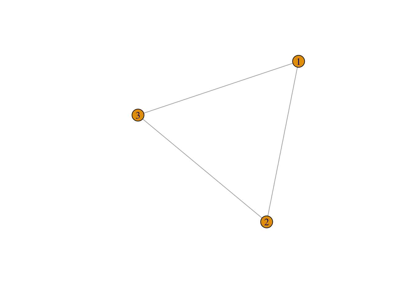

n can be greater than number of vertices in the edge list

g2 <- graph( edges=c(1,2, 2,3, 3,1), n=10 ) # now with 10 vertices, and directed by default
plot(g2)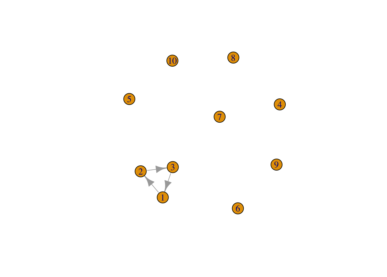

named vertices

g3 <- graph( c("John", "Jim", "Jim", "Jill", "Jill", "John")) 
# When the edge list has vertex names, the number of nodes is not needed
plot(g3)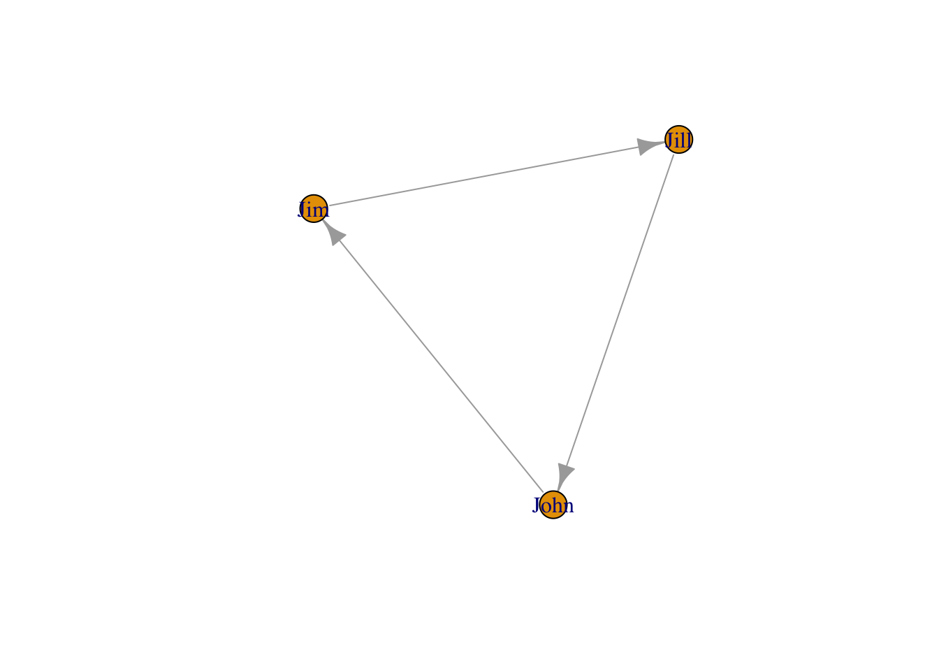

named vertices without edges

g4 <- graph( c("John", "Jim", "Jim", "Jack", "Jim", "Jack", "John", "John"), 
             isolates=c("Jesse", "Janis", "Jennifer", "Justin") )  
# In named graphs we can specify isolates by providing a list of their names.
set.seed(1)
plot(g4, edge.arrow.size=.5, vertex.color="gold", vertex.size=15, 
     vertex.frame.color="gray", vertex.label.color="black", 
     vertex.label.cex=1.5, vertex.label.dist=2, edge.curved=0.2)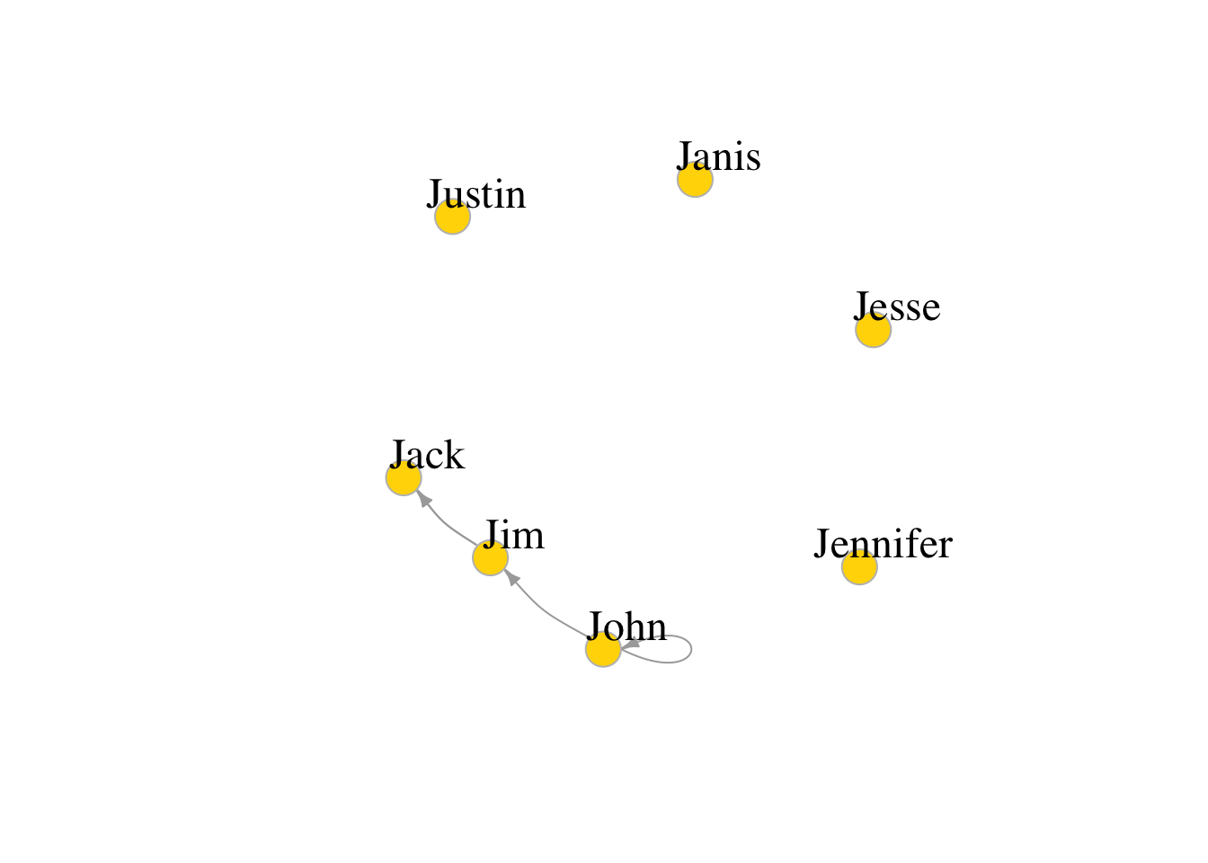

2.2.2.2 `graph_from_literal`

Small graphs can also be generated with a description of this kind:

‘-’ for undirected tie, “+-’ or”-+" for directed ties pointing left & right,
“++” for a symmetric tie, and “:” for sets of vertices

plot(graph_from_literal(a---b, b---c)) # the number of dashes doesn't matter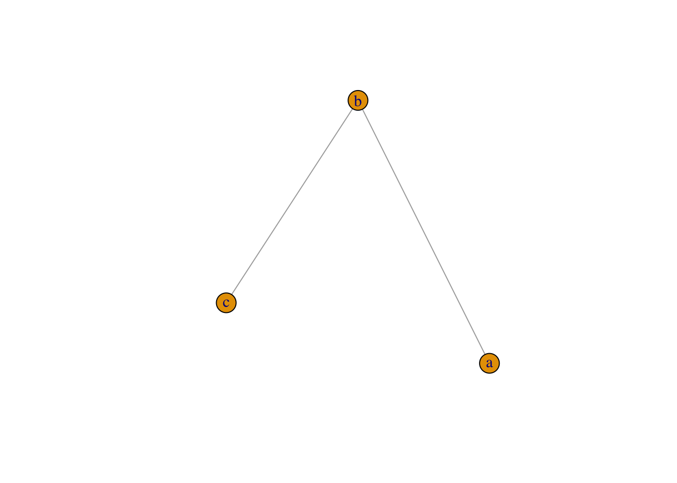

plot(graph_from_literal(a--+b, b+--c))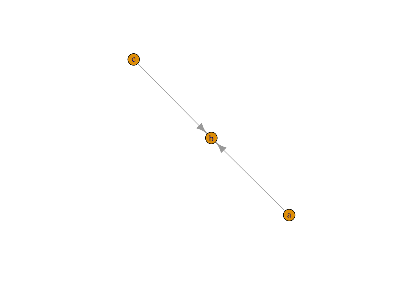

plot(graph_from_literal(a+-+b, b+-+c))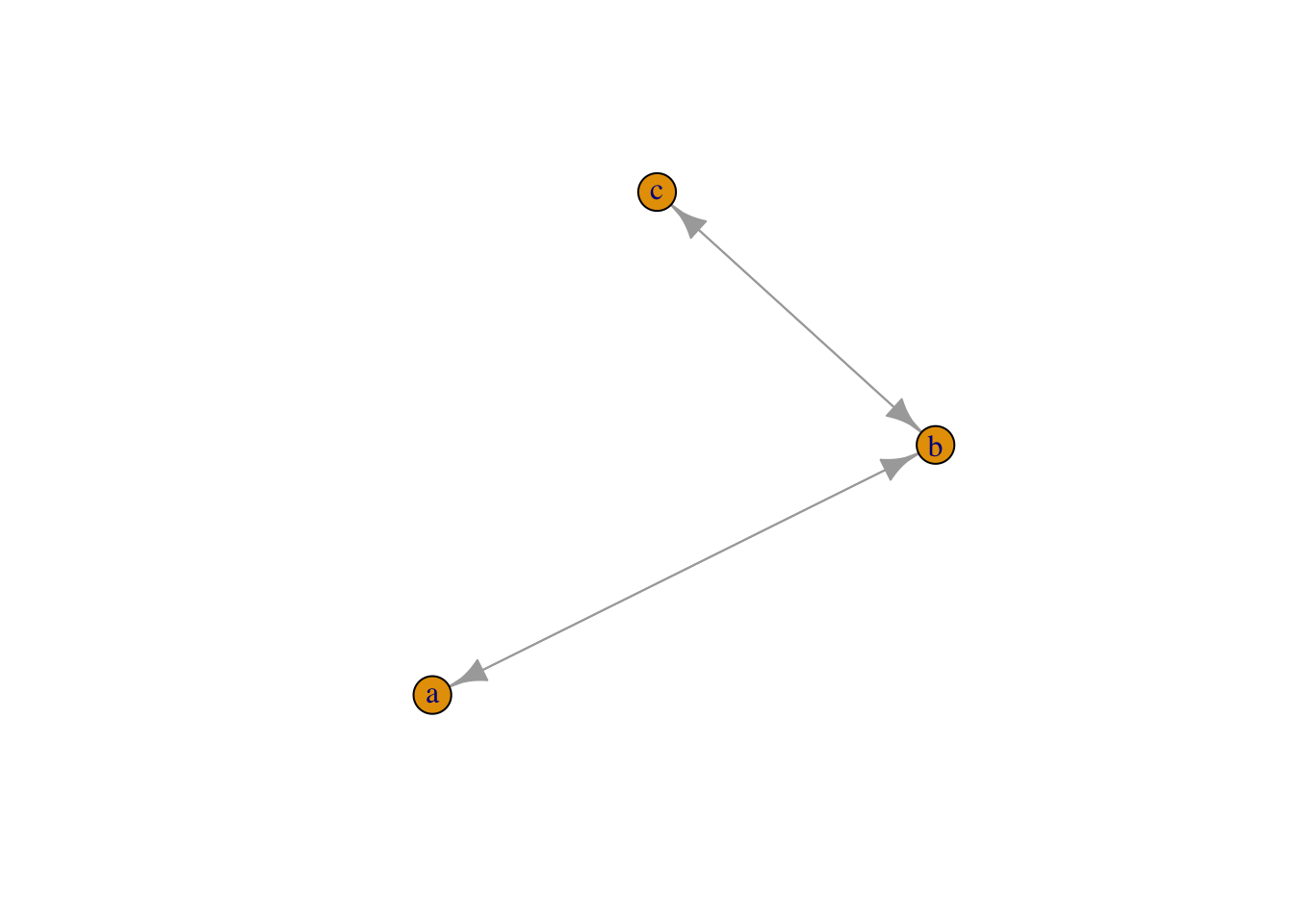

a:b:c using colon to connect abc as a whole group. Each vertex within group a:b:c is connected to each vertex within group c:d:e

plot(graph_from_literal(a:b:c---c:d:e))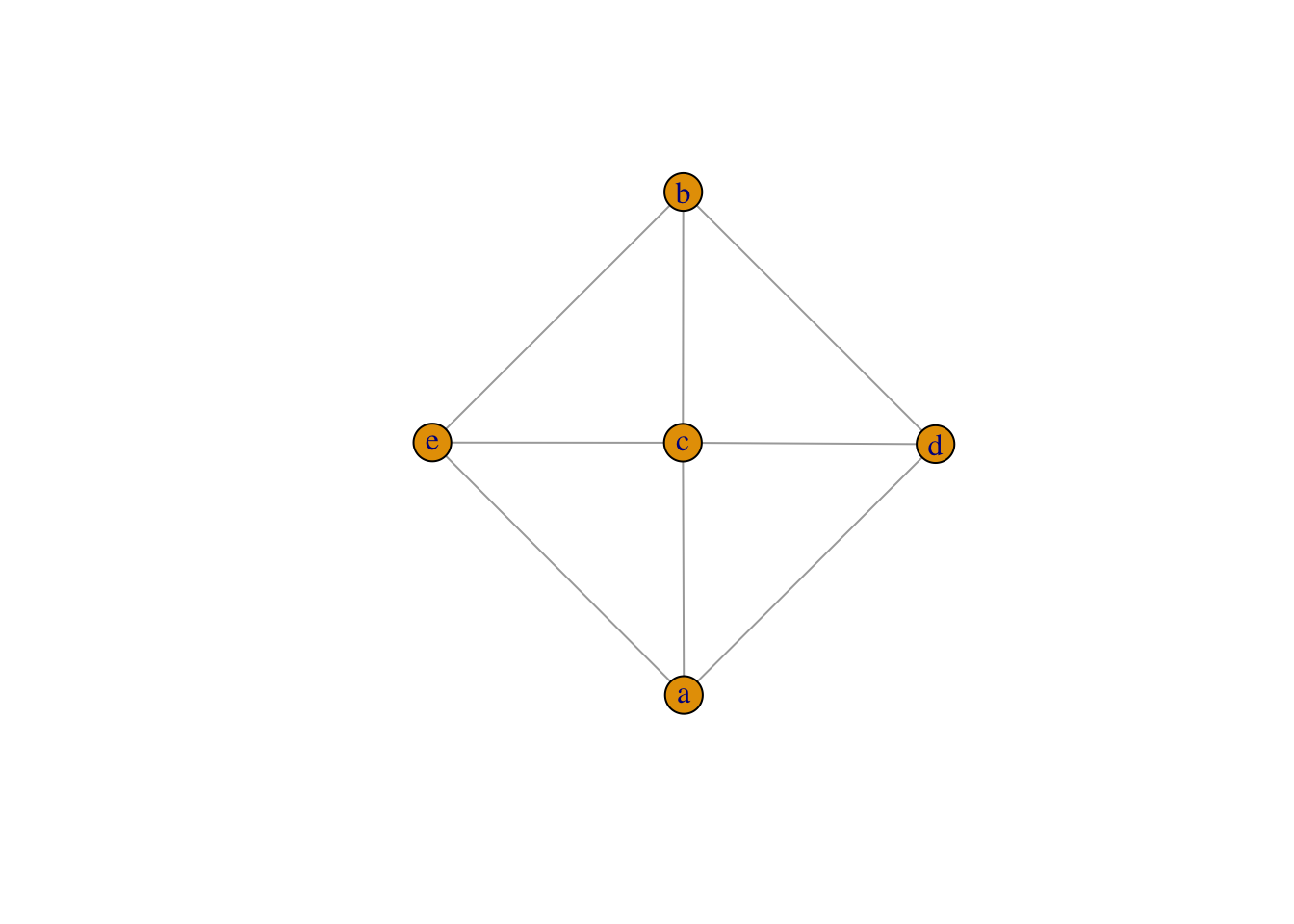

plot(graph_from_literal(a--b:c:d))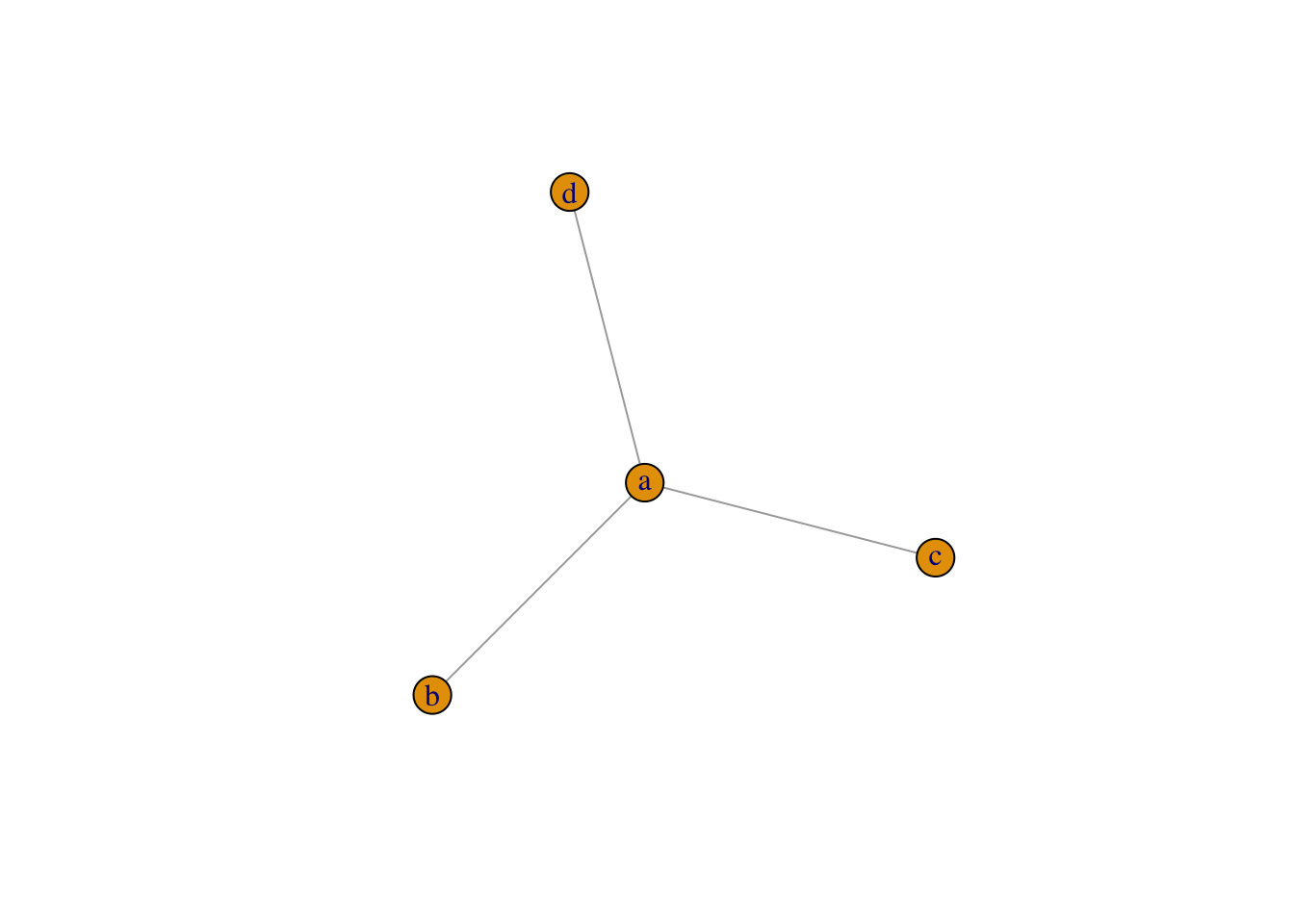

plot(graph_from_literal(a:e--b:c:d))

2.2.3 Creating specific graphs and graph models

Specific graph
- make_empty_graph
- make_full_graph
- make_tree
- make_star
- make_ring
Graph models
- sample_gnm Erdos-Renyi random graph
- sample_gnp Erdos-Renyi with G(n,p) specification
- sample_smallworld Watts-Strogatz small-world model
- sample_pa Barabasi-Albert preferential attachment model for scale-free graphs

2.2.3.1 Empty graph

eg <- make_empty_graph(40)
plot(eg, vertex.size=10, vertex.label=NA)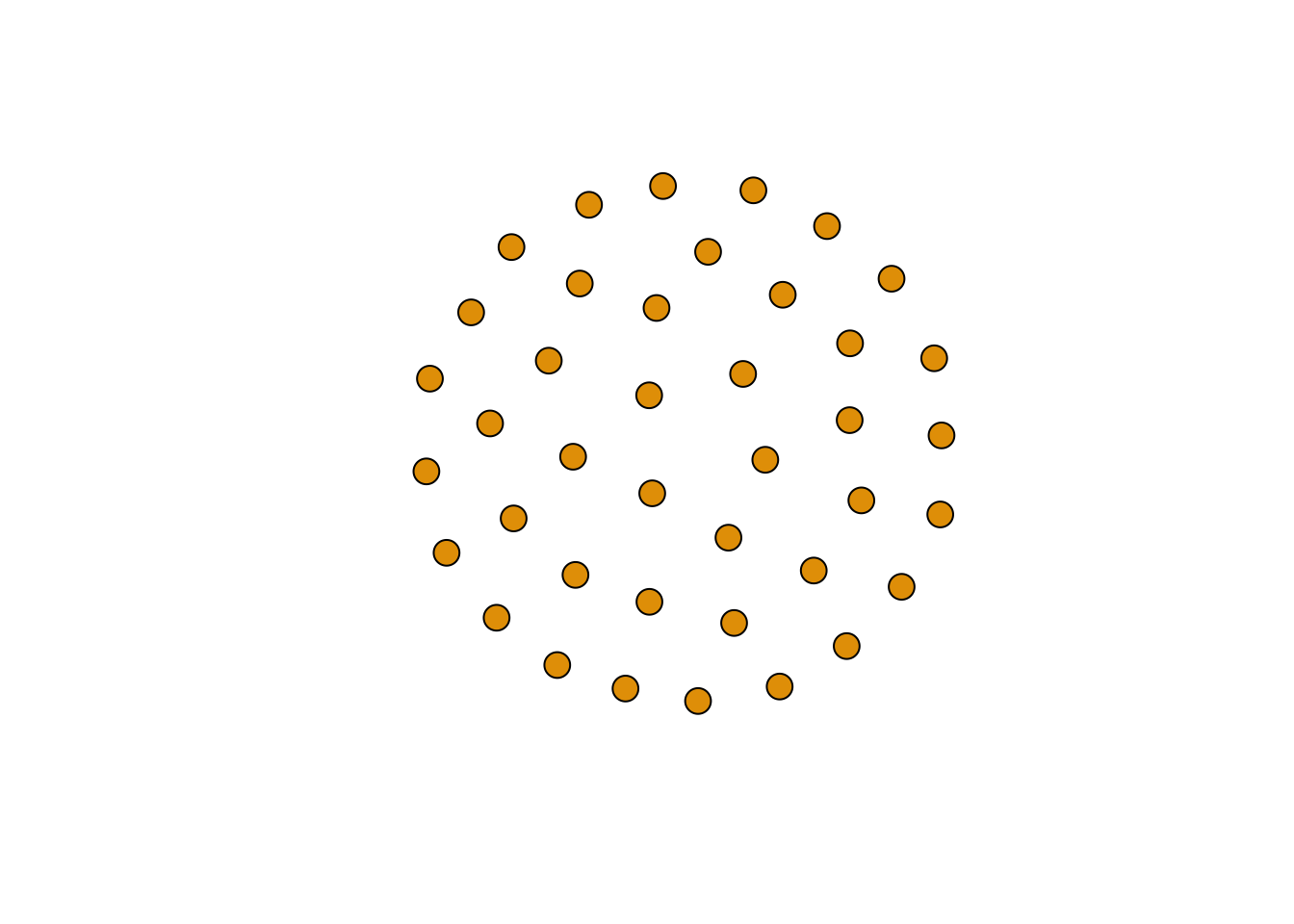

2.2.3.2 Full graph

fg <- make_full_graph(40)
plot(fg, vertex.size=10, vertex.label=NA)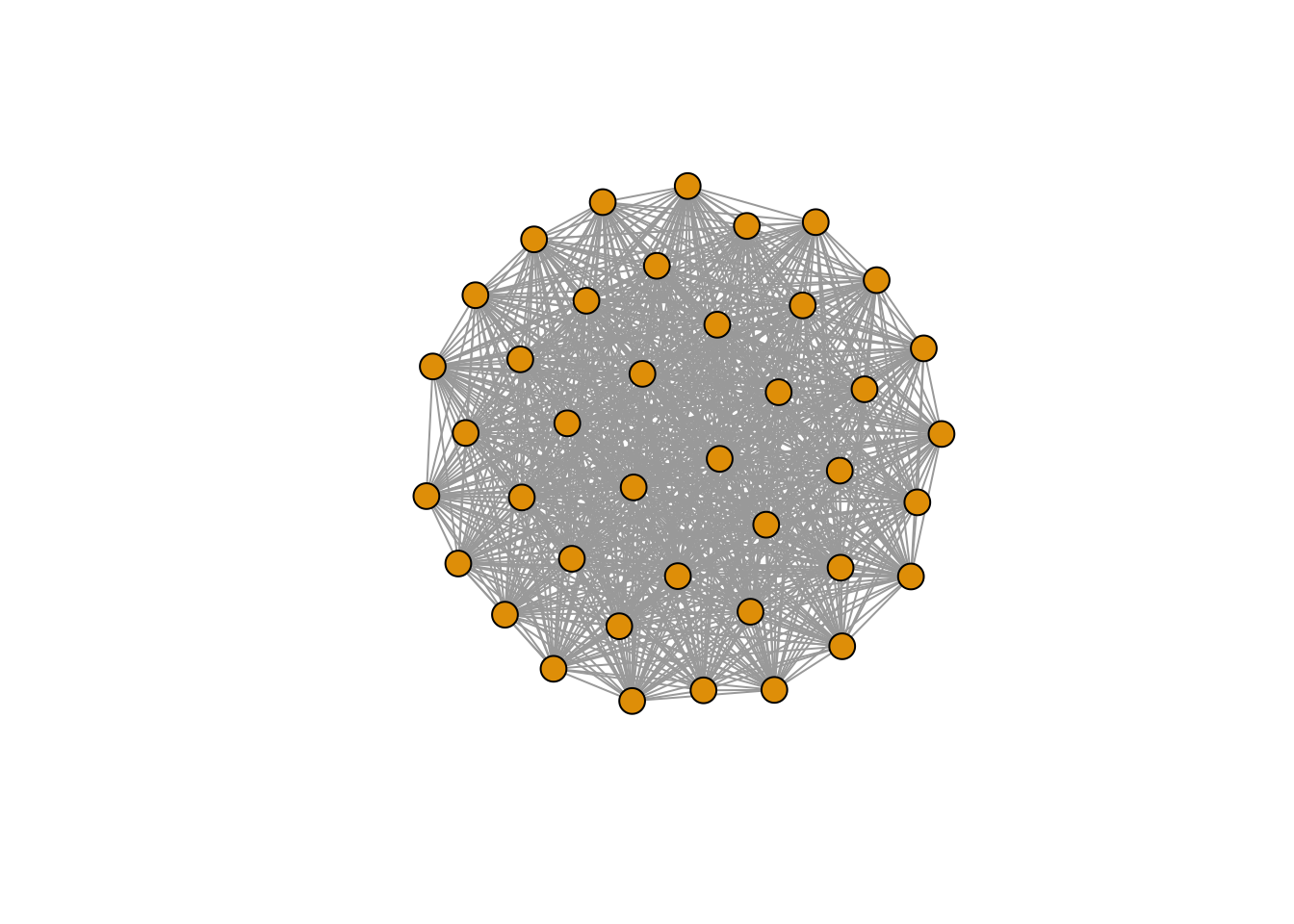

2.2.3.3 Tree graph

tr <- make_tree(40, children = 3, mode = "undirected")

plot(tr, vertex.size=10, vertex.label=NA)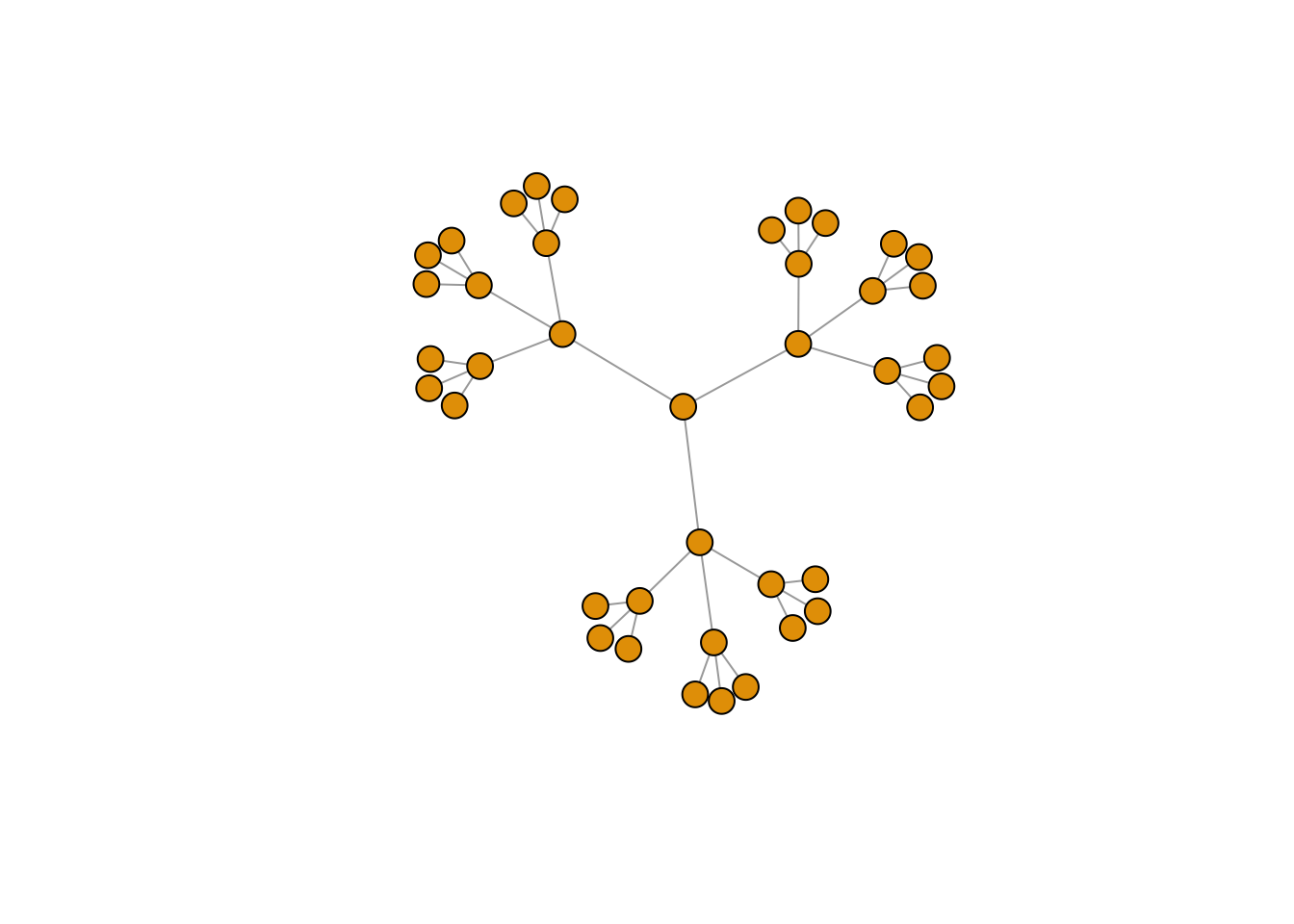

2.2.3.4 Star graph

st <- make_star(40)
plot(st, vertex.size=10, vertex.label=NA)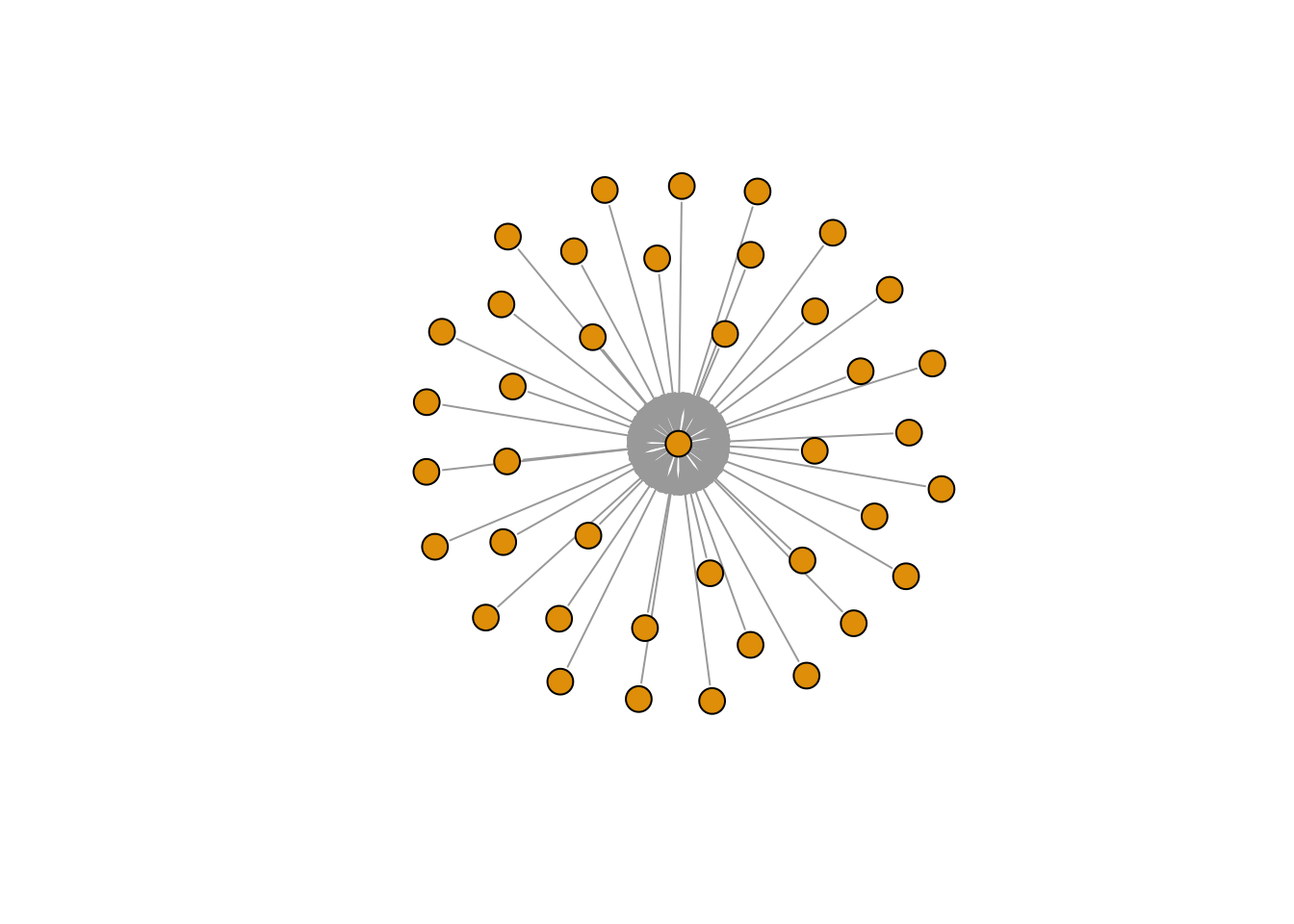

2.2.3.5 Ring graph

rn <- make_ring(40)
plot(rn, vertex.size=10, vertex.label=NA)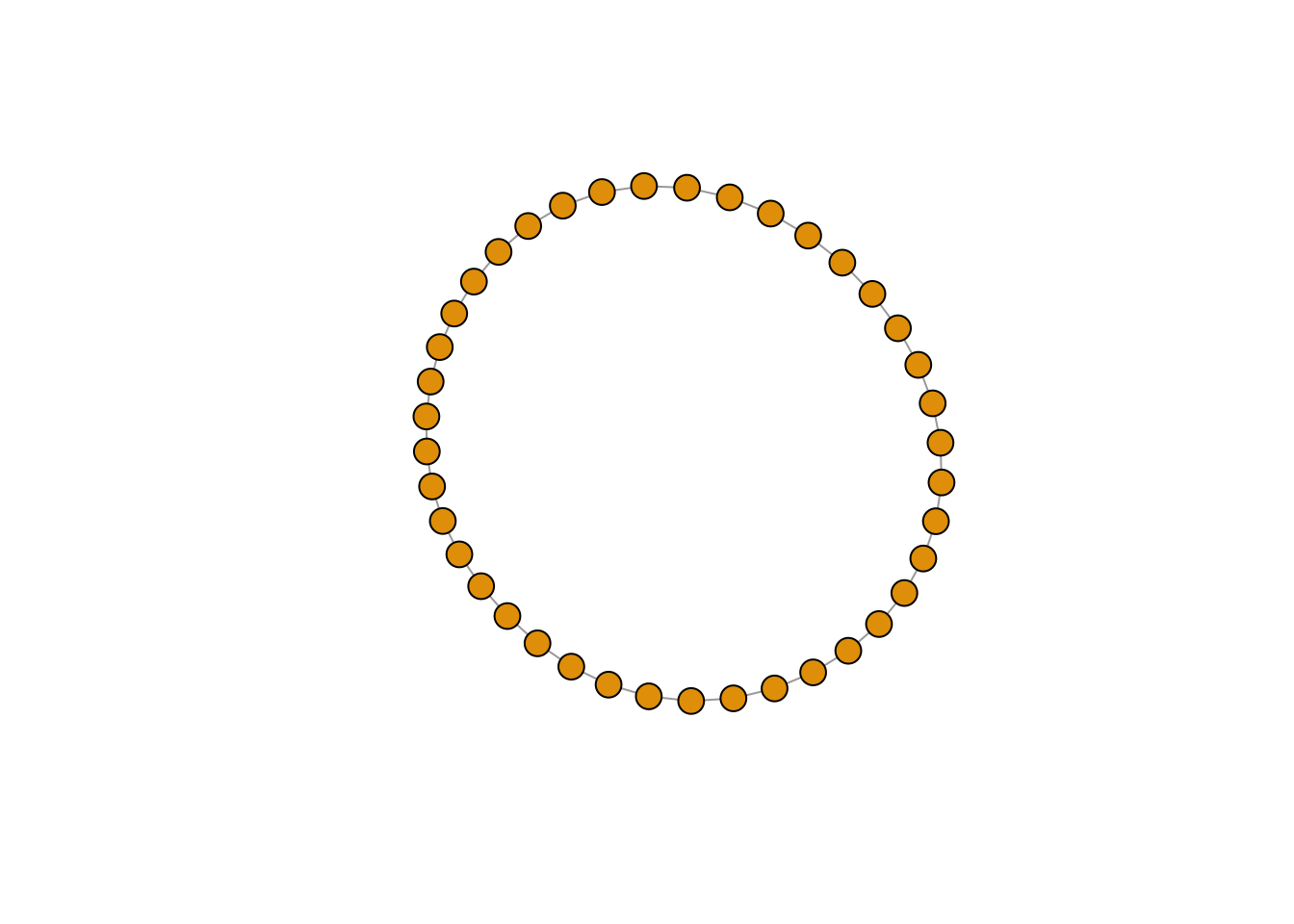

2.2.3.6 Erdos-Renyi random graph

‘n’ is number of nodes, ‘m’ is the number of edges

er <- sample_gnm(n=100, m=40) ####can also use erdos.renyi.game
## options include directed= and loops=
plot(er, vertex.size=6, vertex.label=NA)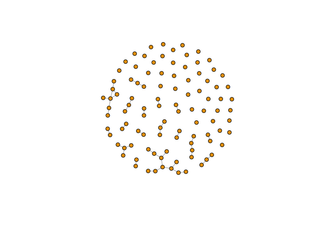

2.2.3.7 Erdos-Renyi with G(n,p) specification

er <- sample_gnp(n=100, p=.02) ####can also use erdos.renyi.game
plot(er, vertex.size=6, vertex.label=NA)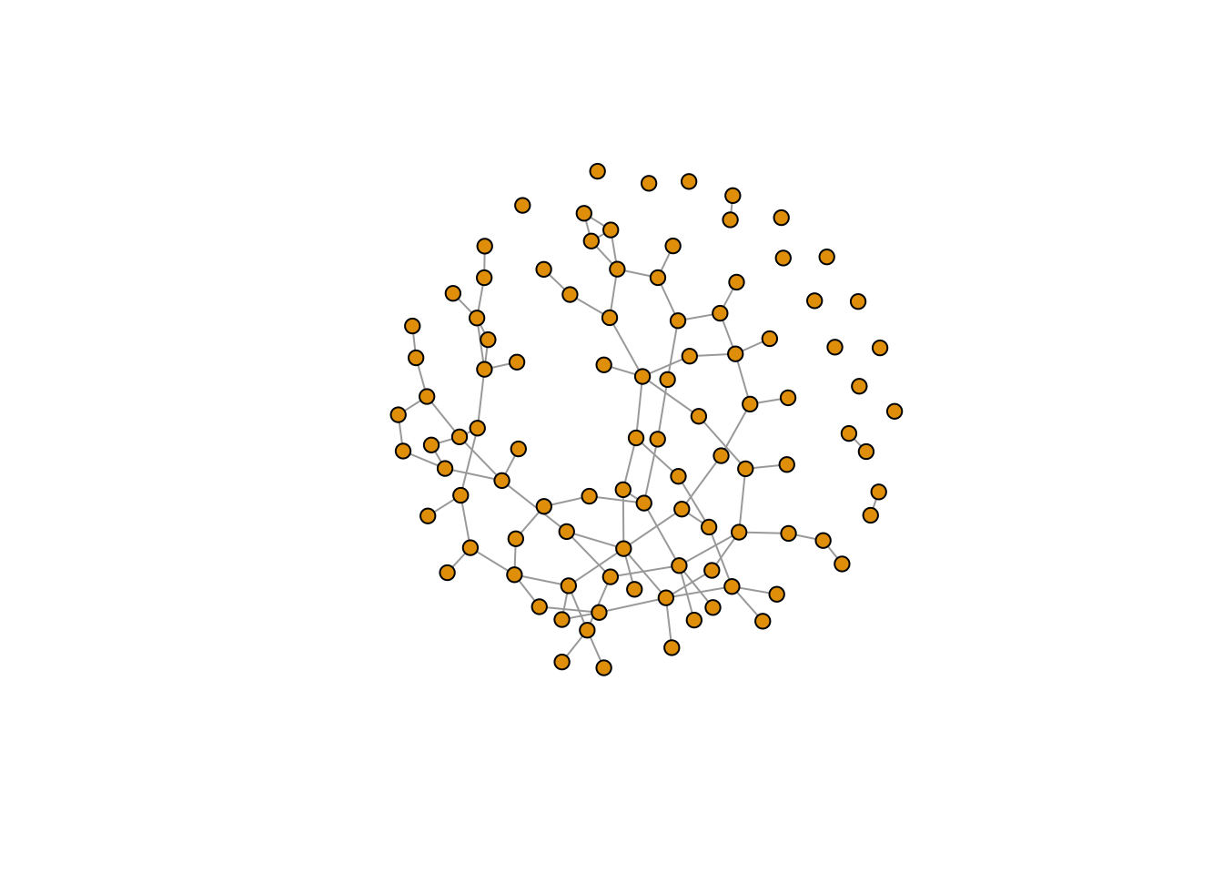

2.2.4 Adjustments on graphs

igraph object as a layer (using +)
igraph object as a matrix (using [])
rewiring a graph using rewire, connect.neighborhood
combine graphs %du%
other functions

2.2.4.1 igraph object as a layer

kite <- make_empty_graph(directed = FALSE) + vertices(LETTERS[1:10]) +
edges('A','B', 'B','D', 'C','D', 'D','E', 'E','G', 'F','G', 'G','H', 'H','I', 'I','J')
plot(kite)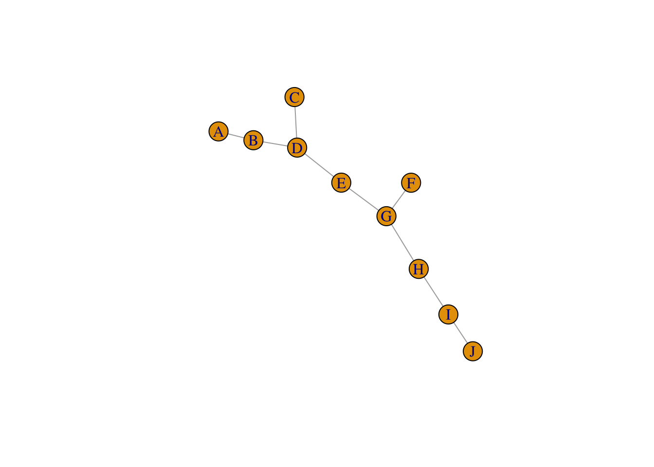

2.2.4.2 igraph object as a matrix

kite[]

## 10 x 10 sparse Matrix of class "dgCMatrix"

##    [[ suppressing 10 column names 'A', 'B', 'C' ... ]]

##                      
## A . 1 . . . . . . . .
## B 1 . . 1 . . . . . .
## C . . . 1 . . . . . .
## D . 1 1 . 1 . . . . .
## E . . . 1 . . 1 . . .
## F . . . . . . 1 . . .
## G . . . . 1 1 . 1 . .
## H . . . . . . 1 . 1 .
## I . . . . . . . 1 . 1
## J . . . . . . . . 1 .

add edge

kite['A','F']=1
kite[]

## 10 x 10 sparse Matrix of class "dgCMatrix"

##    [[ suppressing 10 column names 'A', 'B', 'C' ... ]]

##                      
## A . 1 . . . 1 . . . .
## B 1 . . 1 . . . . . .
## C . . . 1 . . . . . .
## D . 1 1 . 1 . . . . .
## E . . . 1 . . 1 . . .
## F 1 . . . . . 1 . . .
## G . . . . 1 1 . 1 . .
## H . . . . . . 1 . 1 .
## I . . . . . . . 1 . 1
## J . . . . . . . . 1 .

add multiple edges

kite[-1,1]

## B C D E F G H I J 
## 1 0 0 0 1 0 0 0 0

kite[-1,1]=1
kite[] # add multiple edges or using from and to

## 10 x 10 sparse Matrix of class "dgCMatrix"

##    [[ suppressing 10 column names 'A', 'B', 'C' ... ]]

##                      
## A . 1 1 1 1 1 1 1 1 1
## B 1 . . 1 . . . . . .
## C 1 . . 1 . . . . . .
## D 1 1 1 . 1 . . . . .
## E 1 . . 1 . . 1 . . .
## F 1 . . . . . 1 . . .
## G 1 . . . 1 1 . 1 . .
## H 1 . . . . . 1 . 1 .
## I 1 . . . . . . 1 . 1
## J 1 . . . . . . . 1 .

add multiple edges using from and to

kite[from=LETTERS[1:3],to=LETTERS[4:6]]=1
kite[]

## 10 x 10 sparse Matrix of class "dgCMatrix"

##    [[ suppressing 10 column names 'A', 'B', 'C' ... ]]

##                      
## A . 1 1 1 1 1 1 1 1 1
## B 1 . . 1 1 . . . . .
## C 1 . . 1 . 1 . . . .
## D 1 1 1 . 1 . . . . .
## E 1 1 . 1 . . 1 . . .
## F 1 . 1 . . . 1 . . .
## G 1 . . . 1 1 . 1 . .
## H 1 . . . . . 1 . 1 .
## I 1 . . . . . . 1 . 1
## J 1 . . . . . . . 1 .

remove edge

kite[-1,2]=0

2.2.4.3 rewiring a graph

set.seed(1)
plot(rn, vertex.size=10, vertex.label=NA)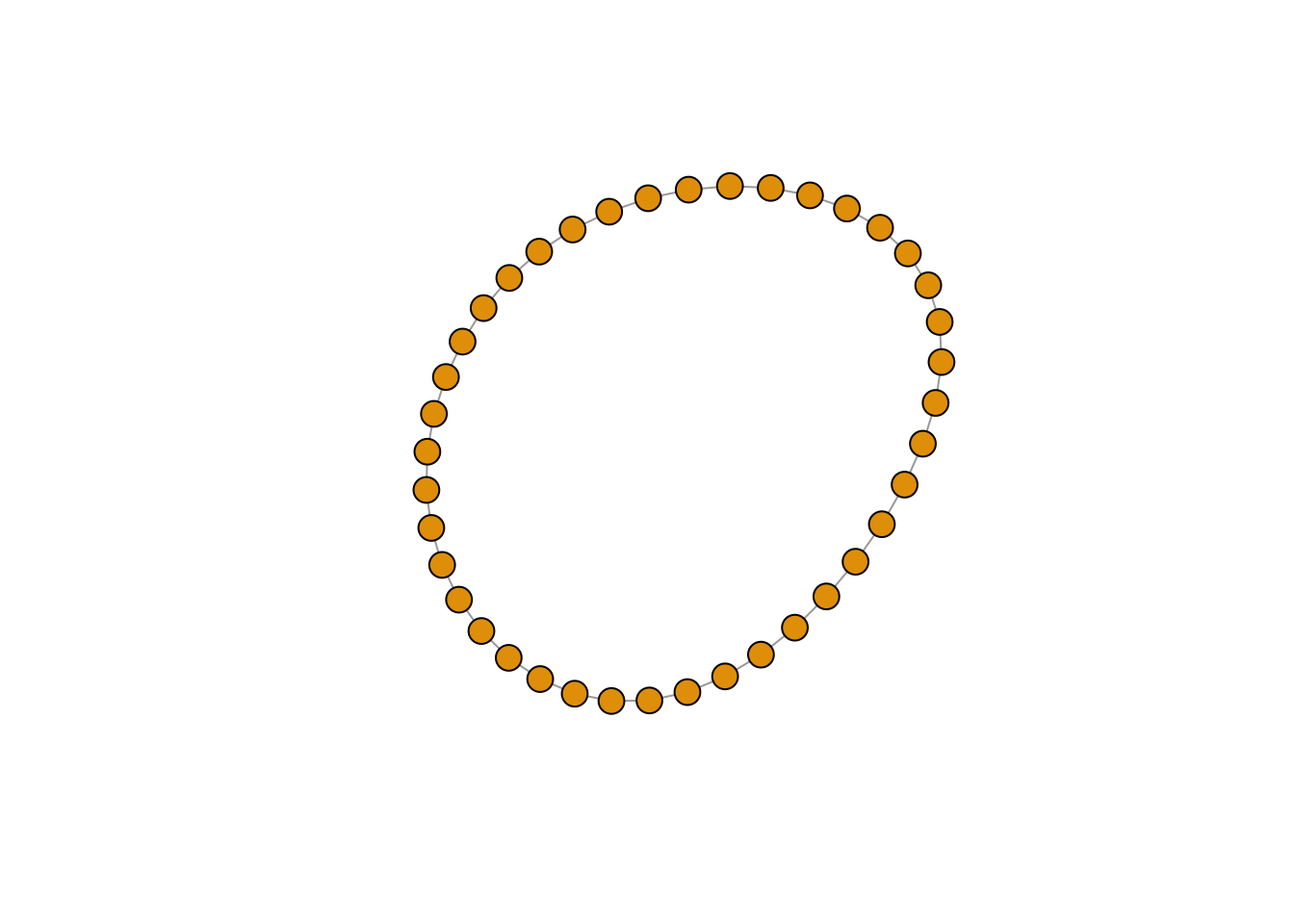

‘each_edge()’ is a rewiring method that changes the edge endpoints to a new vertex with a probability ‘prob’. And the new vertex is random variable distributed uniformly.

rn.rewired <- rewire(rn, each_edge(prob=0.1))
plot(rn.rewired, vertex.size=10, vertex.label=NA)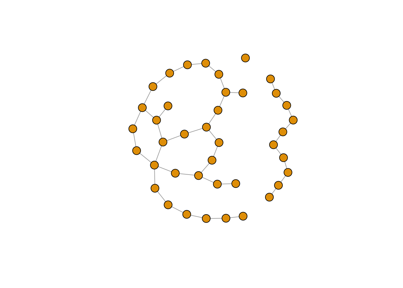

Rewire to connect vertices to other vertices at a certain distance.

rn.neigh = connect.neighborhood(rn, 5)
plot(rn.neigh, vertex.size=8, vertex.label=NA)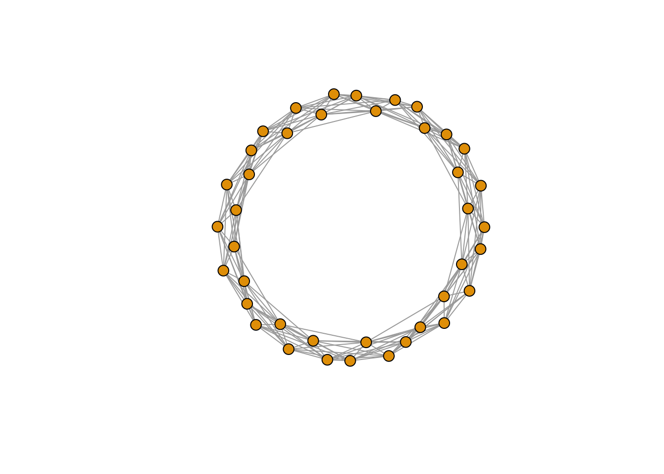

g <- make_ring(10)
plot(g)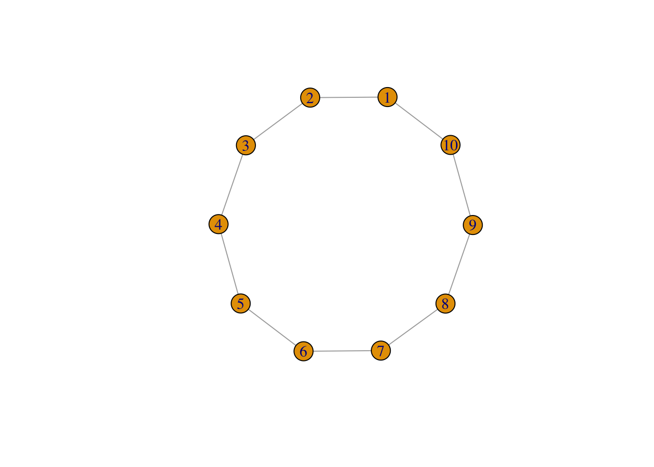

g <- connect(g, 2)
plot(g)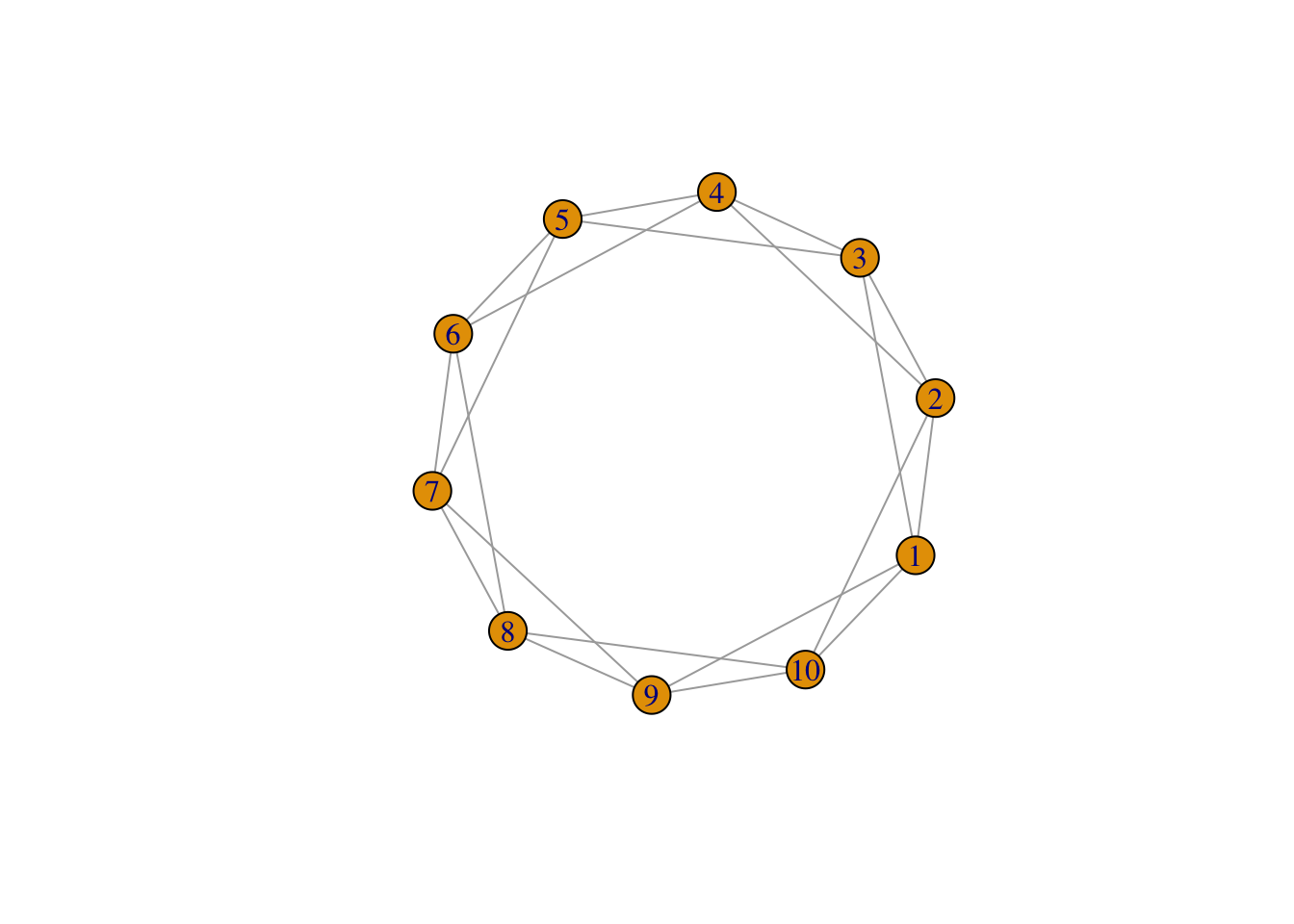

combine graphs

plot(rn %du% tr, vertex.size=10, vertex.label=NA)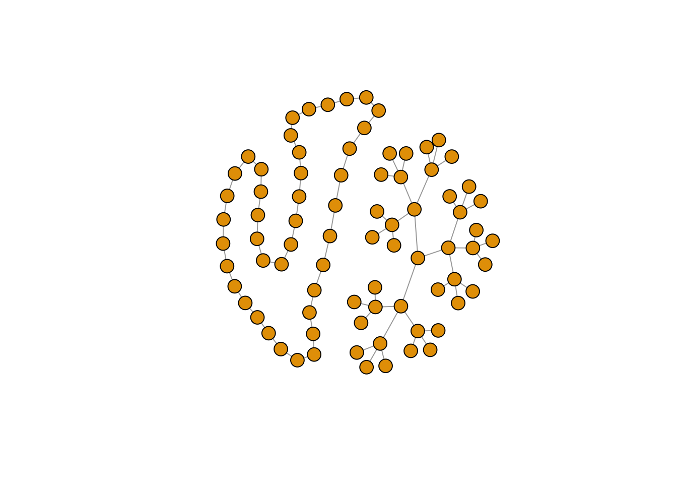

2.2.5 Edge, vertex and network attributes

Consider edge, vertex as sequences []
Consider the network as matrix []
Neighbors [[]]
Attributes $

2.2.5.1 consider edge, vertex as sequences

plot(g4)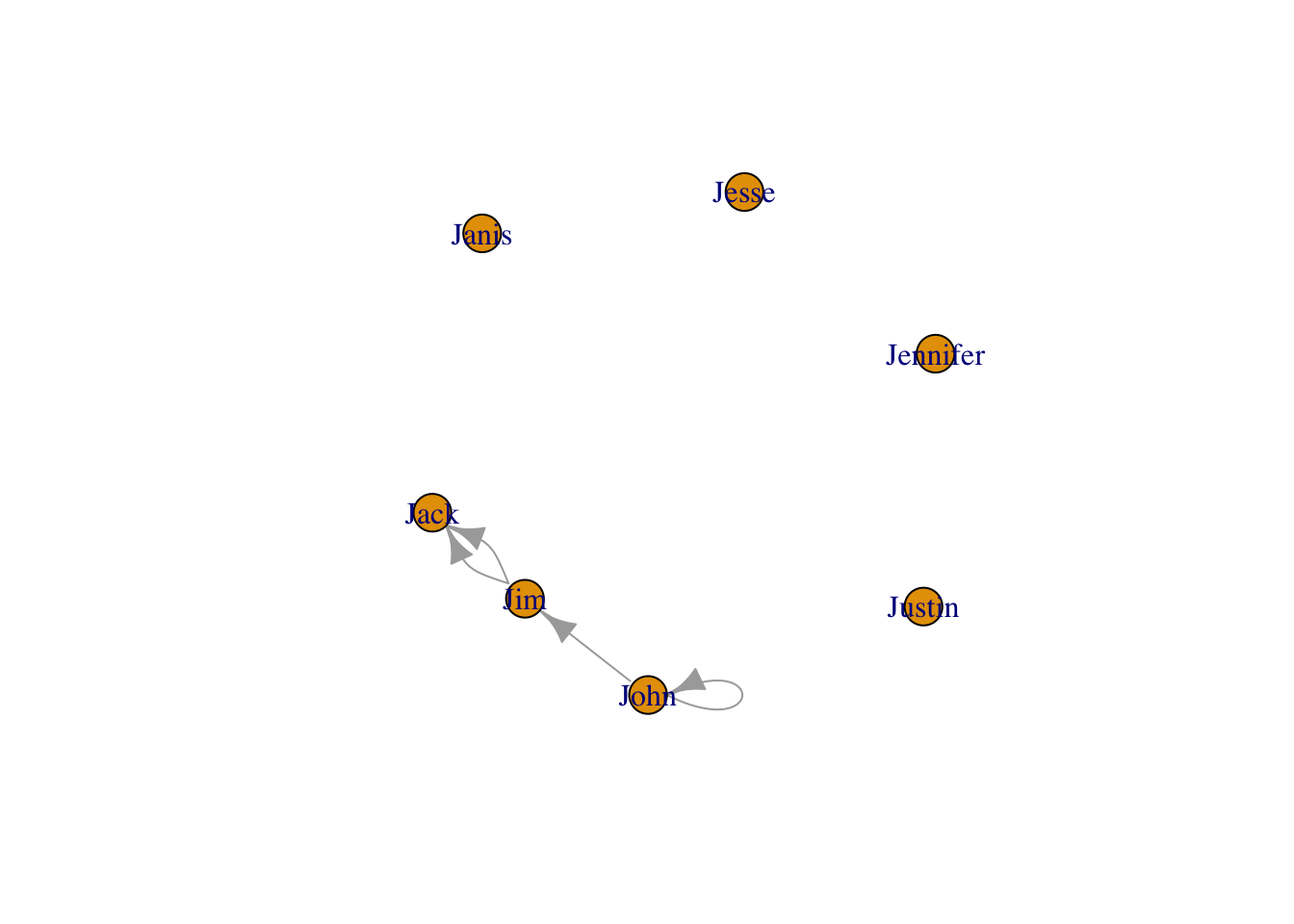

E(g4) #edge list

## + 4/4 edges from 562dd0e (vertex names):
## [1] John->Jim  Jim ->Jack Jim ->Jack John->John

V(g4) #vertex list

## + 7/7 vertices, named, from 562dd0e:
## [1] John     Jim      Jack     Jesse    Janis    Jennifer Justin

ecount(g4) # count

## [1] 4

vcount(g4) # count

## [1] 7

refer vertex and edges

V(g4)[c("John","Jim")]

## + 2/7 vertices, named, from 562dd0e:
## [1] John Jim

V(g4)[nei("Jim")] # neighbors of Jim

## + 2/7 vertices, named, from 562dd0e:
## [1] John Jack

E(g4)[c("John|Jim","Jim|Jack")]

## + 2/4 edges from 562dd0e (vertex names):
## [1] John->Jim  Jim ->Jack

E(g4,path = c("John","Jim","Jack"))

## + 2/4 edges from 562dd0e (vertex names):
## [1] John->Jim  Jim ->Jack

E(g4)[ "John" %--% "Jack" ]

## + 0/4 edges from 562dd0e (vertex names):

E(g4)[ "Jim" %->% "Jack" ]

## + 2/4 edges from 562dd0e (vertex names):
## [1] Jim->Jack Jim->Jack

E(g4)[ from("Jim") ]

## + 2/4 edges from 562dd0e (vertex names):
## [1] Jim->Jack Jim->Jack

E(g4)[ to("Jim") ]

## + 1/4 edge from 562dd0e (vertex names):
## [1] John->Jim

2.2.5.2 consider the network as matrix

class(g4)

## [1] "igraph"

g4[] #"adjacency matrix"

## 7 x 7 sparse Matrix of class "dgCMatrix"
##          John Jim Jack Jesse Janis Jennifer Justin
## John        1   1    .     .     .        .      .
## Jim         .   .    2     .     .        .      .
## Jack        .   .    .     .     .        .      .
## Jesse       .   .    .     .     .        .      .
## Janis       .   .    .     .     .        .      .
## Jennifer    .   .    .     .     .        .      .
## Justin      .   .    .     .     .        .      .

g4[1,] # consider as a matrix to select

##     John      Jim     Jack    Jesse    Janis Jennifer   Justin 
##        1        1        0        0        0        0        0

get.adjacency(g4)

## 7 x 7 sparse Matrix of class "dgCMatrix"
##          John Jim Jack Jesse Janis Jennifer Justin
## John        1   1    .     .     .        .      .
## Jim         .   .    2     .     .        .      .
## Jack        .   .    .     .     .        .      .
## Jesse       .   .    .     .     .        .      .
## Janis       .   .    .     .     .        .      .
## Jennifer    .   .    .     .     .        .      .
## Justin      .   .    .     .     .        .      .

##explicitly getting adjacency matrix (as a sparse matrix)
get.adjacency(g4,sparse=FALSE)

##          John Jim Jack Jesse Janis Jennifer Justin
## John        1   1    0     0     0        0      0
## Jim         0   0    2     0     0        0      0
## Jack        0   0    0     0     0        0      0
## Jesse       0   0    0     0     0        0      0
## Janis       0   0    0     0     0        0      0
## Jennifer    0   0    0     0     0        0      0
## Justin      0   0    0     0     0        0      0

##explicitly getting adjacency matrix  --- not sparse, lets you manipulate it better

g4[1:2,2:3]

## 2 x 2 sparse Matrix of class "dgCMatrix"
##      Jim Jack
## John   1    .
## Jim    .    2

g4[from=c("Jack","Jim","John"),to=c("Jim","Jack","John")]

## [1] 0 1 1

2.2.5.3 neighbors

neighbors(g4,"Jim")

## + 2/7 vertices, named, from 562dd0e:
## [1] Jack Jack

g4[["Jim"]]

## $Jim
## + 2/7 vertices, named, from 562dd0e:
## [1] Jack Jack

g4[[c("Jim","John")]] #works for multiple vertices

## $Jim
## + 2/7 vertices, named, from 562dd0e:
## [1] Jack Jack
## 
## $John
## + 2/7 vertices, named, from 562dd0e:
## [1] John Jim

g4[["Jim",]]

## $Jim
## + 2/7 vertices, named, from 562dd0e:
## [1] Jack Jack

g4[[,"Jim"]]

## $Jim
## + 1/7 vertex, named, from 562dd0e:
## [1] John

g4[[,"Jim",edges=TRUE]]

## $Jim
## + 1/4 edge from 562dd0e (vertex names):
## [1] John->Jim

2.2.5.4 Attributes: vertex attributes, edge attributes, graph attributes

use $ to create attributes and get attributes

V(g4)$name # automatically generated when we created the network.

## [1] "John"     "Jim"      "Jack"     "Jesse"    "Janis"    "Jennifer"
## [7] "Justin"

V(g4)$gender <- c("male", "male", "male", "male", "female", "female", "male")
neighbors(g4,"Jim",mode = "all")$gender

## [1] "male" "male" "male"

E(g4)$type <- "email" # Edge attribute, assign "email" to all edges
E(g4)$weight <- 10    # Edge weight, setting all existing edges to 10
g4 <- set_graph_attr(g4, "name", "Email Network")

see the attributes

edge_attr(g4)

## $type
## [1] "email" "email" "email" "email"
## 
## $weight
## [1] 10 10 10 10

vertex_attr(g4)

## $name
## [1] "John"     "Jim"      "Jack"     "Jesse"    "Janis"    "Jennifer"
## [7] "Justin"  
## 
## $gender
## [1] "male"   "male"   "male"   "male"   "female" "female" "male"

graph_attr(g4)

## $name
## [1] "Email Network"

graph_attr_names(g4)

## [1] "name"

graph_attr(g4, "name")

## [1] "Email Network"

can remove the attribute

g4 <- set_graph_attr(g4, "something", "A thing")
g4 <- delete_graph_attr(g4, "something")
graph_attr(g4)

## $name
## [1] "Email Network"

Make use of these attributes

plot(g4, edge.arrow.size=.5, vertex.label.color="black", vertex.label.dist=1.5,
     vertex.color=as.factor(V(g4)$gender) )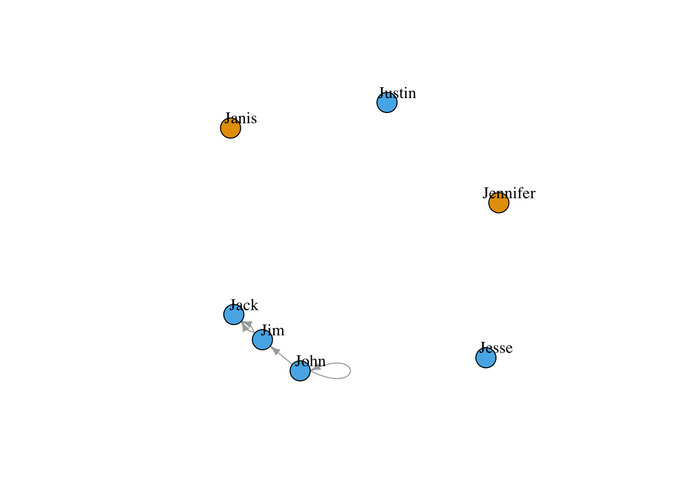

plot(g4, edge.arrow.size=.5, vertex.label.color="black", vertex.label.dist=1.5,
     vertex.color=c( "pink", "skyblue")[1+(V(g4)$gender=="male")] )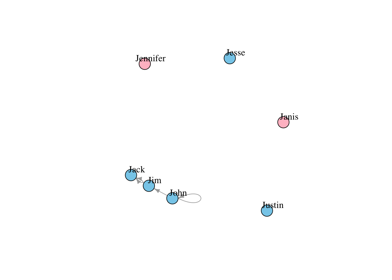

#consider as a sequence

attributes can be combined

plot(g4)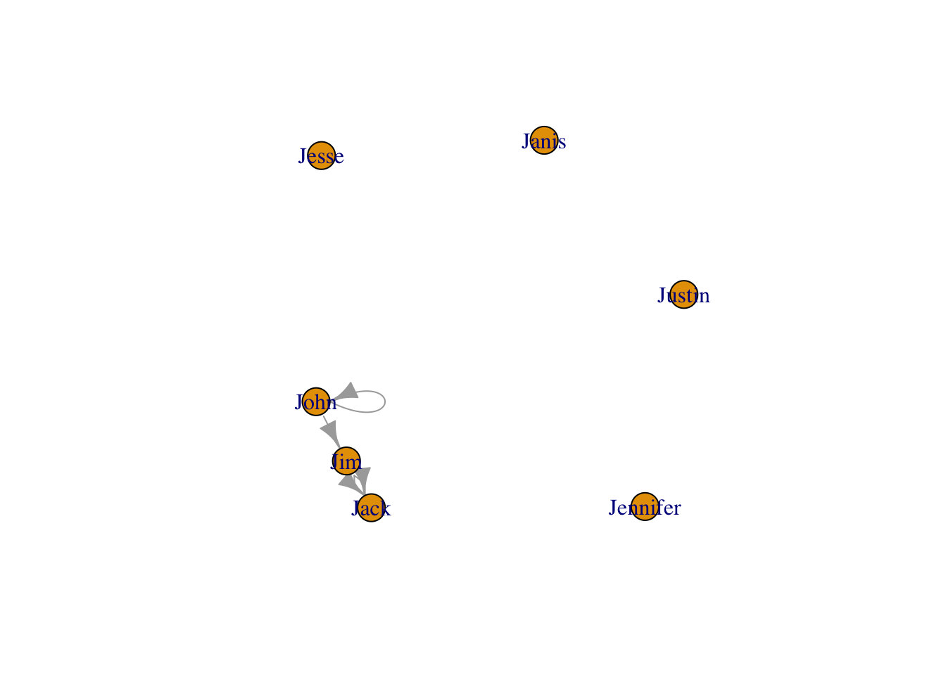

g4s <- igraph::simplify( g4, remove.multiple = T, remove.loops = F, 
                 edge.attr.comb=c(weight="sum", type="ignore") )
#specifies what to do with edge attributes, if remove.multiple=TRUE. In this case many edges might be mapped to a single one in the new graph, and their attributes are combined.
E(g4)$type

## [1] "email" "email" "email" "email"

E(g4s)$type

## NULL

E(g4)$weight

## [1] 10 10 10 10

E(g4s)$weight

## [1] 10 10 20

2.2.5.5 special attributes

make sure to avoid using these attribute names: color(e/v), layout(g), name(v),shape(v),type(v),weight(e)

2.2.6 Description of igraph object

g4s

## IGRAPH 6cadc8c DNW- 7 3 -- Email Network
## + attr: name (g/c), name (v/c), gender (v/c), weight (e/n)
## + edges from 6cadc8c (vertex names):
## [1] John->John John->Jim  Jim ->Jack

D or U, for a directed or undirected graph
N for a named graph (where nodes have a name attribute)
W for a weighted graph (where edges have a weight attribute)
B for a bipartite (two-mode) graph (where nodes have a type attribute)
(7 5) refer to the number of nodes and edges
node & edge attributes, for example: g:graph; v: vertex; e: edge;n:numeric; c:character;l:logical; x:complex

data(karate)
karate

## IGRAPH 4b458a1 UNW- 34 78 -- Zachary's karate club network
## + attr: name (g/c), Citation (g/c), Author (g/c), Faction (v/n),
## | name (v/c), label (v/c), color (v/n), weight (e/n)
## + edges from 4b458a1 (vertex names):
##  [1] Mr Hi  --Actor 2  Mr Hi  --Actor 3  Mr Hi  --Actor 4 
##  [4] Mr Hi  --Actor 5  Mr Hi  --Actor 6  Mr Hi  --Actor 7 
##  [7] Mr Hi  --Actor 8  Mr Hi  --Actor 9  Mr Hi  --Actor 11
## [10] Mr Hi  --Actor 12 Mr Hi  --Actor 13 Mr Hi  --Actor 14
## [13] Mr Hi  --Actor 18 Mr Hi  --Actor 20 Mr Hi  --Actor 22
## [16] Mr Hi  --Actor 32 Actor 2--Actor 3  Actor 2--Actor 4 
## [19] Actor 2--Actor 8  Actor 2--Actor 14 Actor 2--Actor 18
## + ... omitted several edges

data(macaque)
macaque

## IGRAPH f7130f3 DN-- 45 463 -- 
## + attr: Citation (g/c), Author (g/c), shape (v/c), name (v/c)
## + edges from f7130f3 (vertex names):
##  [1] V1 ->V2     V1 ->V3     V1 ->V3A    V1 ->V4     V1 ->V4t   
##  [6] V1 ->MT     V1 ->PO     V1 ->PIP    V2 ->V1     V2 ->V3    
## [11] V2 ->V3A    V2 ->V4     V2 ->V4t    V2 ->VOT    V2 ->VP    
## [16] V2 ->MT     V2 ->MSTd/p V2 ->MSTl   V2 ->PO     V2 ->PIP   
## [21] V2 ->VIP    V2 ->FST    V2 ->FEF    V3 ->V1     V3 ->V2    
## [26] V3 ->V3A    V3 ->V4     V3 ->V4t    V3 ->MT     V3 ->MSTd/p
## [31] V3 ->PO     V3 ->LIP    V3 ->PIP    V3 ->VIP    V3 ->FST   
## [36] V3 ->TF     V3 ->FEF    V3A->V1     V3A->V2     V3A->V3    
## + ... omitted several edges

2.3 Built networks from external sources, basic visualization and more on network descriptions

2.3.1 Outline

Get network from files (edgelist, matrix, dataframe)
Visualization
- Plotting parameters
- Layouts
Network and node descriptions

2.3.2 Dataset

Datasets: Download the data from my github.
The full dataset comes from https://github.com/mathbeveridge/asoiaf
Analysis on the datasets: https://www.macalester.edu/~abeverid/thrones.html

Network Visualization from [abeverid](https://www.macalester.edu/~abeverid/thrones.html)

Figure 2.2: Network Visualization from abeverid

2.3.3 Get network from files

2.3.3.1 Creating network

Introduction from [`igraph` manual](https://sites.fas.harvard.edu/~airoldi/pub/books/BookDraft-CsardiNepuszAiroldi2016.pdf)

Figure 2.3: Introduction from igraph manual

Figure 2.4: Introduction from igraph manual

Figure 2.5: Introduction from igraph manual

Figure 2.6: Introduction from igraph manual

Figure 2.7: Introduction from igraph manual

2.3.3.2 Get network from files

graph_from_adjacency_matrix()
graph_from_edgelist()
graph_from_data_frame()

2.3.3.3 `graph_from_adjacency_matrix()`

Used for creating a small matrix.

The networks in real world are usually large sparse matrix and stored as a edgelist.

Binary matrix:

set.seed(2)
#sample from Bernoulli distribution with sample size 100. 
adjm <- matrix(sample(0:1, 100, replace=TRUE, prob=c(0.9,0.1)), nc=10)
adjm

##       [,1] [,2] [,3] [,4] [,5] [,6] [,7] [,8] [,9] [,10]
##  [1,]    0    0    0    0    1    0    0    0    0     1
##  [2,]    0    0    0    0    0    0    0    0    0     0
##  [3,]    0    0    0    0    0    0    0    0    0     0
##  [4,]    0    0    0    0    0    1    0    0    0     0
##  [5,]    1    0    0    0    1    0    0    0    0     0
##  [6,]    1    0    0    0    0    0    0    0    0     0
##  [7,]    0    1    0    0    1    0    0    0    1     0
##  [8,]    0    0    0    0    0    1    0    0    0     0
##  [9,]    0    0    1    0    0    0    0    0    0     0
## [10,]    0    0    0    0    0    0    0    0    0     0

g1 <- graph_from_adjacency_matrix( adjm )
set.seed(1)
plot(g1)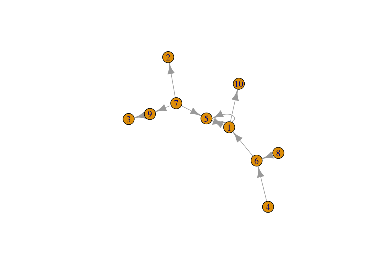

#default is directed
g2 <- graph_from_adjacency_matrix( adjm ,mode = "undirected")
set.seed(1)
plot(g2)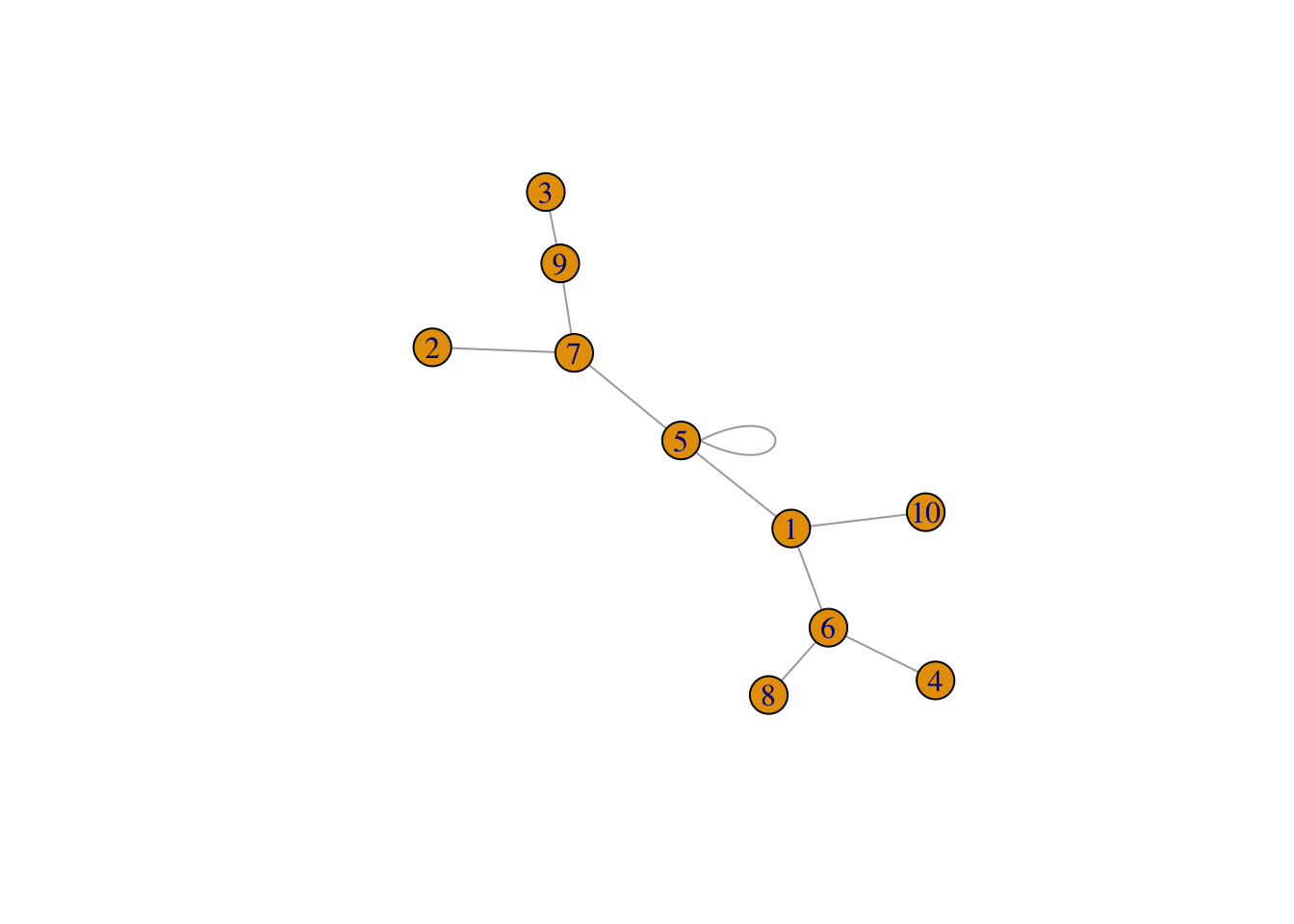

#get rid of the self-loop (in real-world maybe self-loop does not make any sense)
g3 <- graph_from_adjacency_matrix( adjm ,mode = "undirected",diag = FALSE)
set.seed(1)
plot(g3)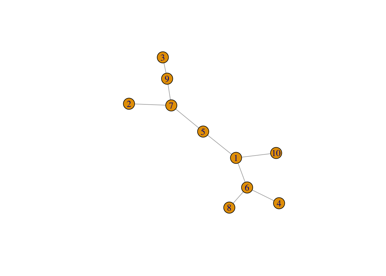

Sparse matrix:

adjms=g1[]
adjms

## 10 x 10 sparse Matrix of class "dgCMatrix"
##                          
##  [1,] . . . . 1 . . . . 1
##  [2,] . . . . . . . . . .
##  [3,] . . . . . . . . . .
##  [4,] . . . . . 1 . . . .
##  [5,] 1 . . . 1 . . . . .
##  [6,] 1 . . . . . . . . .
##  [7,] . 1 . . 1 . . . 1 .
##  [8,] . . . . . 1 . . . .
##  [9,] . . 1 . . . . . . .
## [10,] . . . . . . . . . .

g4=graph_from_adjacency_matrix(adjms)
set.seed(1)
plot(g4)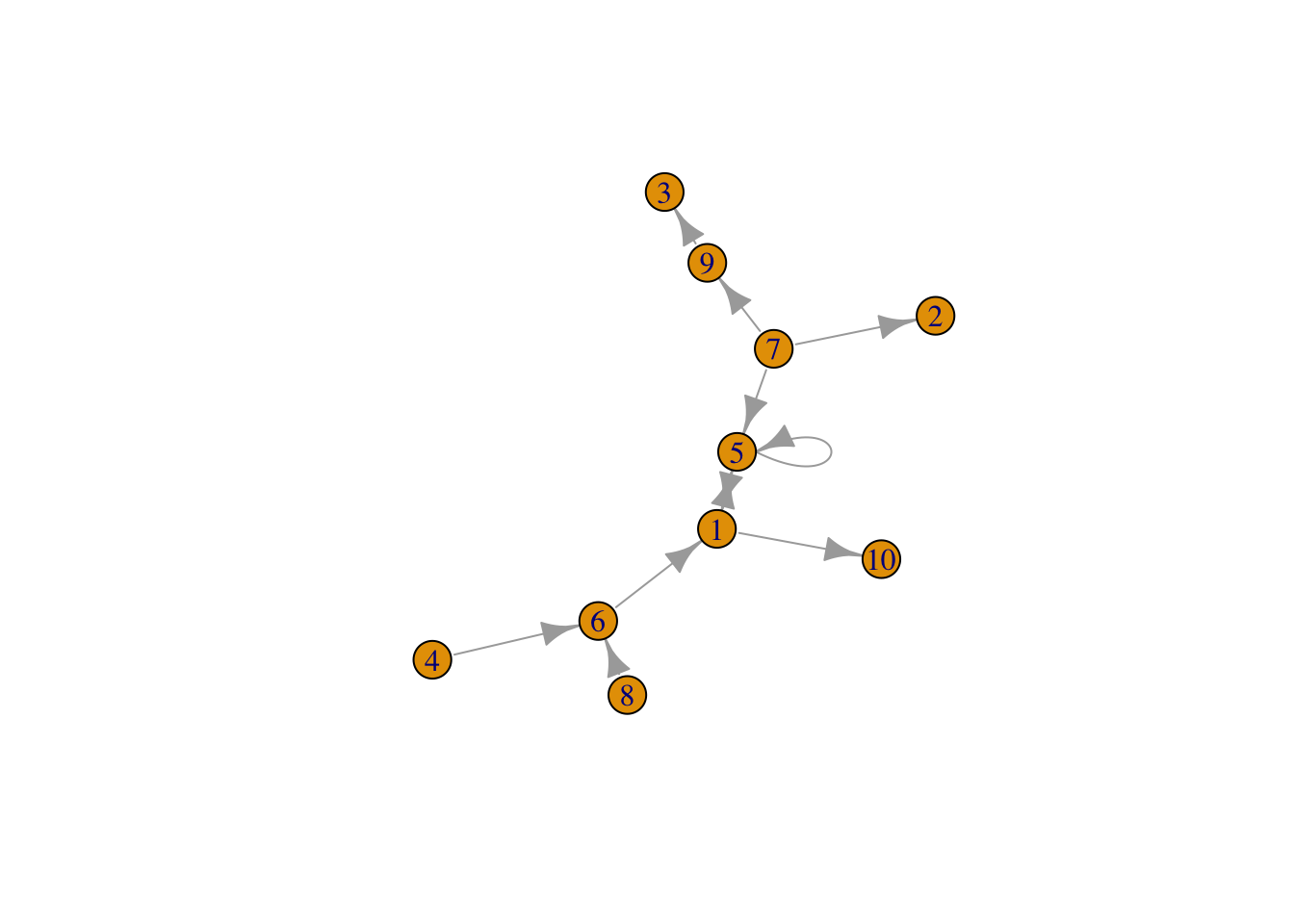

Weighted matrix

set.seed(1)
adjmw <- matrix(sample(0:5, 100, replace=TRUE,
                      prob=c(0.9,0.02,0.02,0.02,0.02,0.02)), nc=10)
adjmw

##       [,1] [,2] [,3] [,4] [,5] [,6] [,7] [,8] [,9] [,10]
##  [1,]    0    0    3    0    0    0    2    0    0     0
##  [2,]    0    0    0    0    0    0    0    0    0     0
##  [3,]    0    0    0    0    0    0    0    0    0     0
##  [4,]    2    0    0    0    0    0    0    0    0     0
##  [5,]    0    0    0    0    0    0    0    0    0     0
##  [6,]    0    0    0    0    0    0    0    0    0     0
##  [7,]    4    0    0    0    0    0    0    0    0     0
##  [8,]    0    1    0    0    0    0    0    0    0     0
##  [9,]    0    0    0    0    0    0    0    0    0     0
## [10,]    0    0    0    0    0    0    0    5    0     0

g5 <- graph_from_adjacency_matrix(adjmw, weighted=TRUE)
set.seed(1)
plot(g5)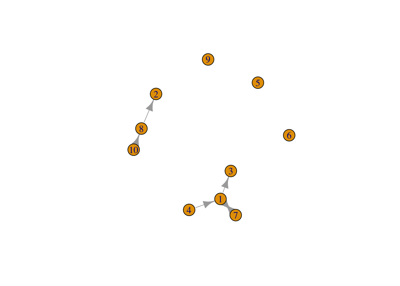

g5

## IGRAPH 6f0feb3 D-W- 10 6 -- 
## + attr: weight (e/n)
## + edges from 6f0feb3:
## [1]  1->3  1->7  4->1  7->1  8->2 10->8

E(g5)$weight

## [1] 3 2 2 4 1 5

Named matrix

rownames(adjmw)=LETTERS[1:10]
colnames(adjmw)=LETTERS[1:10]
g6 <- graph_from_adjacency_matrix(adjmw, weighted=TRUE)
set.seed(1)
plot(g6)

2.3.3.4 `graph_from_edgelist()`

Most network datasets are stored as edgelists. Input is two-column matrix with each row defining one edge.

gotdf=read.csv("images/gotstark_lannister.csv",stringsAsFactors = FALSE)
head(gotdf,5)

##   X     Source           Target       Type weight book source.family
## 1 1 Arya-Stark     Benjen-Stark Undirected      3    1         Stark
## 2 2 Arya-Stark       Bran-Stark Undirected     14    1         Stark
## 3 3 Arya-Stark    Catelyn-Stark Undirected      5    1         Stark
## 4 4 Arya-Stark Cersei-Lannister Undirected     12    1         Stark
## 5 5 Arya-Stark          Desmond Undirected      3    1         Stark
##   target.family
## 1         Stark
## 2         Stark
## 3         Stark
## 4     Lannister
## 5          <NA>

library(dplyr)
library(tidyr)

gotdf.el=gotdf%>%select(Source,Target,weight)%>%
  group_by(Source,Target)%>%
  expand(edge=c(1:weight))%>%select(-edge)
head(gotdf.el)

## # A tibble: 6 x 2
## # Groups:   Source, Target [2]
##   Source     Target      
##   <chr>      <chr>       
## 1 Arya-Stark Benjen-Stark
## 2 Arya-Stark Benjen-Stark
## 3 Arya-Stark Benjen-Stark
## 4 Arya-Stark Bran-Stark  
## 5 Arya-Stark Bran-Stark  
## 6 Arya-Stark Bran-Stark

## input need to be a matrix
got1=graph_from_edgelist(gotdf.el%>%as.matrix(),directed = FALSE)
got1

## IGRAPH bdd718b UN-- 99 3374 -- 
## + attr: name (v/c)
## + edges from bdd718b (vertex names):
##  [1] Arya-Stark--Benjen-Stark  Arya-Stark--Benjen-Stark 
##  [3] Arya-Stark--Benjen-Stark  Arya-Stark--Bran-Stark   
##  [5] Arya-Stark--Bran-Stark    Arya-Stark--Bran-Stark   
##  [7] Arya-Stark--Bran-Stark    Arya-Stark--Bran-Stark   
##  [9] Arya-Stark--Bran-Stark    Arya-Stark--Bran-Stark   
## [11] Arya-Stark--Bran-Stark    Arya-Stark--Bran-Stark   
## [13] Arya-Stark--Bran-Stark    Arya-Stark--Bran-Stark   
## [15] Arya-Stark--Bran-Stark    Arya-Stark--Bran-Stark   
## + ... omitted several edges

plot(got1,edge.arrow.size=.5, vertex.color="gold", vertex.size=3, 
     vertex.frame.color="gray", vertex.label.color="black", 
     vertex.label.cex=.5, vertex.label.dist=2, edge.curved=0.2)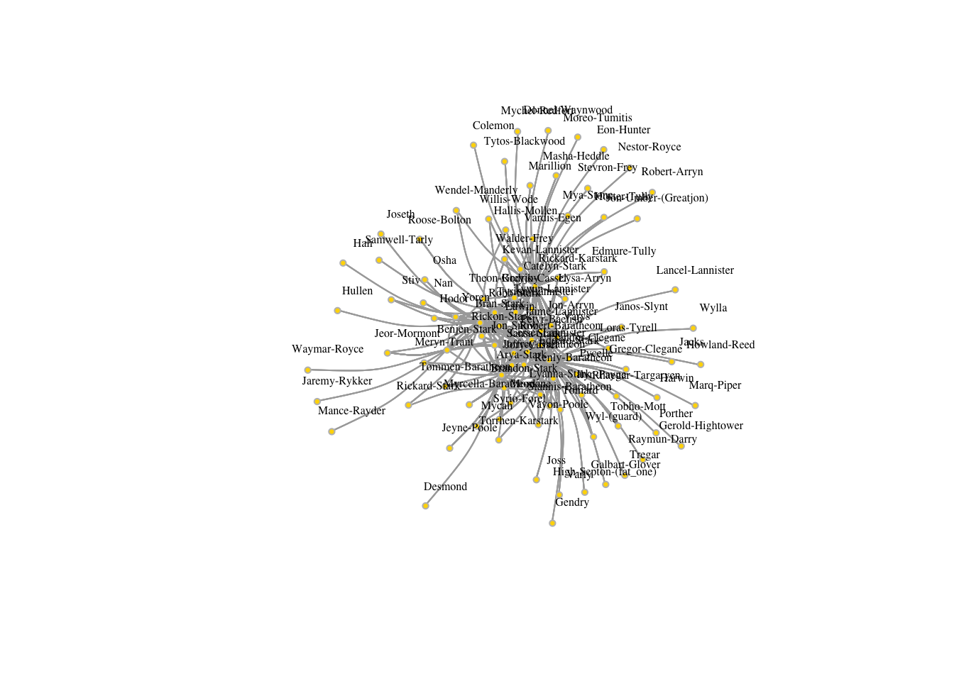

2.3.3.4.1 Simplify the network

el <- matrix( c("foo", "bar","foo","bar", "bar", "foobar"), nc = 2, byrow = TRUE)
graph_from_edgelist(el)%>%plot()

E(got1)$weight=rep(1,ecount(got1))
got1s <- igraph::simplify( got1, remove.multiple = T, remove.loops = F, 
                 edge.attr.comb=c(weight="sum"))
plot(got1s,edge.arrow.size=.5, vertex.color="gold", vertex.size=3, 
     vertex.frame.color="gray", vertex.label.color="black", 
     vertex.label.cex=.5, vertex.label.dist=2, edge.curved=0.5,layout=layout_with_lgl)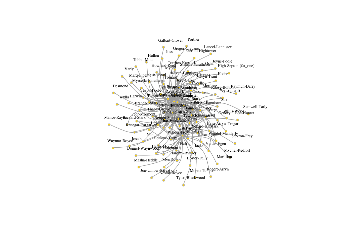

2.3.3.4.2 Short name

library(stringr)

nameshort=V(got1s)$name%>%
  str_split(.,"-",simplify = TRUE)%>%
  .[,1]
V(got1s)$name[1:3]

## [1] "Arya-Stark"   "Benjen-Stark" "Bran-Stark"

nameshort[1:3]

## [1] "Arya"   "Benjen" "Bran"

V(got1s)$name=nameshort
plot(got1s,edge.arrow.size=.5, vertex.color="gold", vertex.size=3, 
     vertex.frame.color="gray", vertex.label.color="black", 
     vertex.label.cex=.5, vertex.label.dist=2, edge.curved=0.5,layout=layout_with_lgl)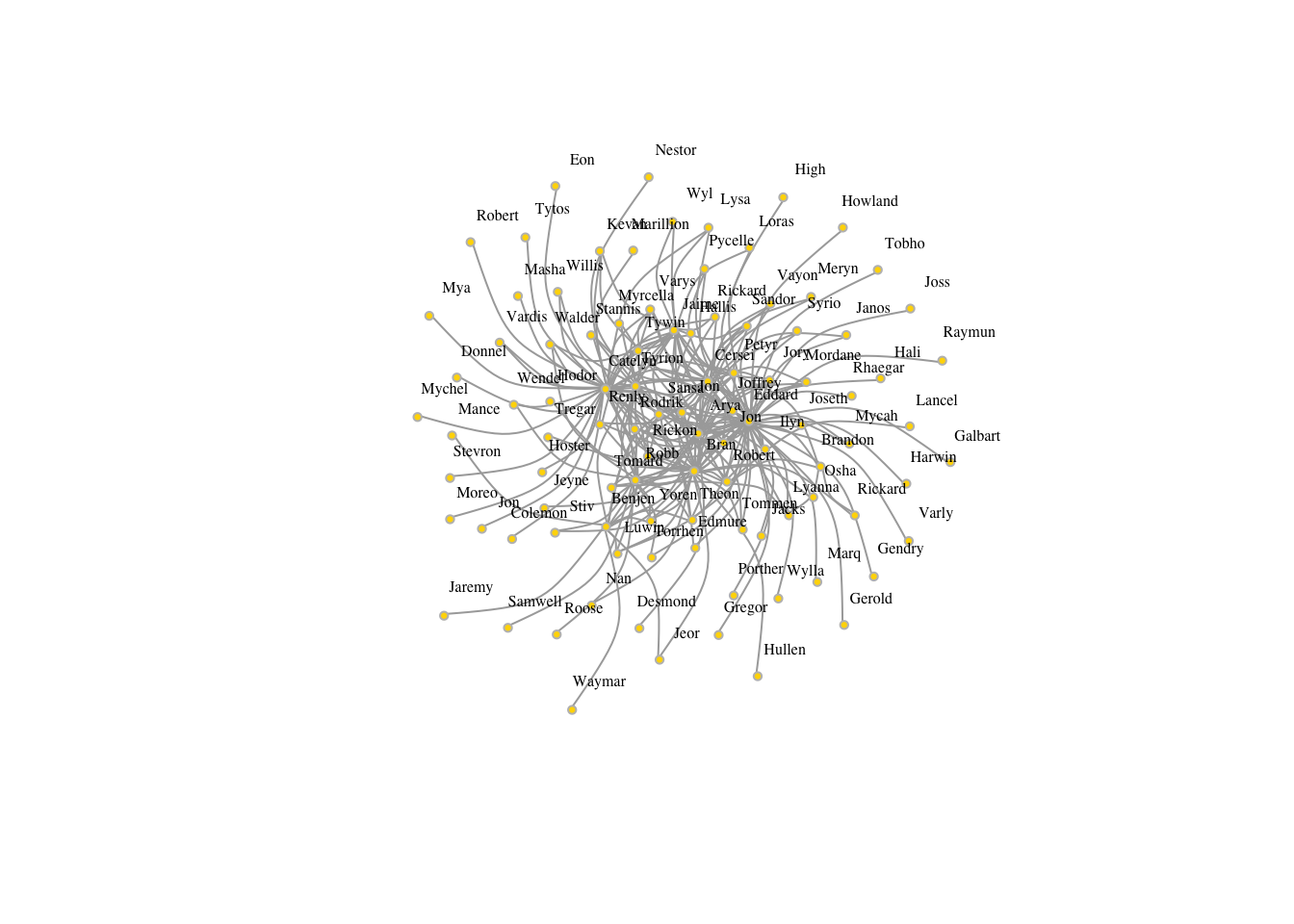

2.3.3.5 `graph_from_data_frame()`

Most common and useful.

d: a data frame containing a symbolic edge list in the first two columns. Additional columns are considered as edge attributes.

vertices: A data frame with vertex metadata

head(gotdf,5)

##   X     Source           Target       Type weight book source.family
## 1 1 Arya-Stark     Benjen-Stark Undirected      3    1         Stark
## 2 2 Arya-Stark       Bran-Stark Undirected     14    1         Stark
## 3 3 Arya-Stark    Catelyn-Stark Undirected      5    1         Stark
## 4 4 Arya-Stark Cersei-Lannister Undirected     12    1         Stark
## 5 5 Arya-Stark          Desmond Undirected      3    1         Stark
##   target.family
## 1         Stark
## 2         Stark
## 3         Stark
## 4     Lannister
## 5          <NA>

gotdf=gotdf%>%select(-X)
got2=graph_from_data_frame(d=gotdf,directed = FALSE)
got2

## IGRAPH 21f2988 UNW- 99 238 -- 
## + attr: name (v/c), Type (e/c), weight (e/n), book (e/n),
## | source.family (e/c), target.family (e/c)
## + edges from 21f2988 (vertex names):
##  [1] Arya-Stark--Benjen-Stark       Arya-Stark--Bran-Stark        
##  [3] Arya-Stark--Catelyn-Stark      Arya-Stark--Cersei-Lannister  
##  [5] Arya-Stark--Desmond            Arya-Stark--Eddard-Stark      
##  [7] Arya-Stark--Ilyn-Payne         Arya-Stark--Jeyne-Poole       
##  [9] Arya-Stark--Joffrey-Baratheon  Arya-Stark--Jon-Snow          
## [11] Arya-Stark--Jory-Cassel        Arya-Stark--Meryn-Trant       
## [13] Arya-Stark--Mordane            Arya-Stark--Mycah             
## + ... omitted several edges

plot(got2,edge.arrow.size=.5, vertex.color="gold", vertex.size=3, 
     vertex.frame.color="gray", vertex.label.color="black", 
     vertex.label.cex=.5, vertex.label.dist=2, edge.curved=0.5,layout=layout_with_lgl)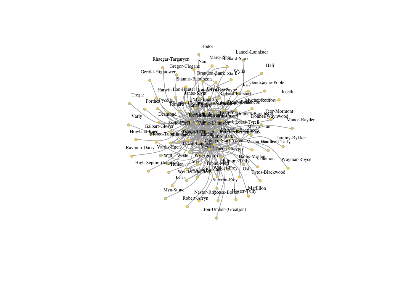

2.3.3.5.1 get dataframe, matrix or adgelist from igraph object

igraph::as_data_frame(got2)%>%head(2)

##         from           to       Type weight book source.family
## 1 Arya-Stark Benjen-Stark Undirected      3    1         Stark
## 2 Arya-Stark   Bran-Stark Undirected     14    1         Stark
##   target.family
## 1         Stark
## 2         Stark

as_adjacency_matrix(got2)%>%head(2)

## [1] 0 1

as_edgelist(got2)%>%head(2)

##      [,1]         [,2]          
## [1,] "Arya-Stark" "Benjen-Stark"
## [2,] "Arya-Stark" "Bran-Stark"

2.3.3.5.2 `read_graph`, `write_graph`

## store in txt or csv or others 
write_graph(graph = got2,file = "g.txt",format = "edgelist")
read_graph(file = "g.txt",format = "edgelist",directed=F)

## IGRAPH 99ad3df U--- 99 238 -- 
## + edges from 99ad3df:
##   [1] 1-- 2 1-- 3 1-- 5 1-- 6 1-- 7 1--12 1--13 1--14 1--17 1--18 1--19
##  [12] 1--20 1--21 1--22 1--23 1--24 1--25 1--26 1--27 1--28 1--29 1--30
##  [23] 1--31 1--32 1--33 1--34 1--35 2-- 3 2-- 6 2--13 2--15 2--21 2--28
##  [34] 2--35 2--36 2--37 2--38 2--39 2--40 2--41 3-- 5 3-- 6 3-- 7 3--12
##  [45] 3--13 3--14 3--15 3--20 3--21 3--22 3--27 3--28 3--29 3--33 3--35
##  [56] 3--37 3--38 3--40 3--42 3--43 3--44 3--45 3--46 3--47 3--48 3--49
##  [67] 3--50 3--51 3--52 3--53 4-- 7 4--11 4--27 4--28 4--52 5-- 6 5-- 7
##  [78] 5-- 8 5--12 5--13 5--14 5--15 5--16 5--20 5--21 5--27 5--28 5--29
##  [89] 5--38 5--40 5--43 5--46 5--51 5--54 5--55 5--56 5--57 5--58 5--59
## + ... omitted several edges

## store the whole graph
write_graph(got2,file = "gg",format = "pajek")
read_graph(file="gg",format="pajek")

## IGRAPH 6586ad6 U-W- 99 238 -- 
## + attr: weight (e/n)
## + edges from 6586ad6:
##  [1] 1-- 2 1-- 3 1-- 5 1-- 6 1--17 1-- 7 1--18 1--19 1--20 1--21 1--22
## [12] 1--23 1--24 1--25 1--26 1--27 1--12 1--13 1--28 1--29 1--30 1--14
## [23] 1--31 1--32 1--33 1--34 1--35 2-- 3 2-- 6 2--36 2--37 2--21 2--38
## [34] 2--39 2--13 2--28 2--40 2--15 2--41 2--35 3-- 5 3-- 6 3-- 7 3--42
## [45] 3--43 3--44 3--45 3--37 3--20 3--46 3--21 3--22 3--47 3--38 3--48
## [56] 3--49 3--27 3--50 3--51 3--52 3--12 3--13 3--28 3--29 3--14 3--53
## [67] 3--40 3--33 3--15 3--35 4-- 7 4--11 4--27 4--52 4--28 5-- 6 5--54
## [78] 5--55 5-- 7 5--56 5--57 5--43 5--58 5-- 8 5--20 5--46 5--21 5--59
## + ... omitted several edges

got2

## IGRAPH 21f2988 UNW- 99 238 -- 
## + attr: name (v/c), Type (e/c), weight (e/n), book (e/n),
## | source.family (e/c), target.family (e/c)
## + edges from 21f2988 (vertex names):
##  [1] Arya-Stark--Benjen-Stark       Arya-Stark--Bran-Stark        
##  [3] Arya-Stark--Catelyn-Stark      Arya-Stark--Cersei-Lannister  
##  [5] Arya-Stark--Desmond            Arya-Stark--Eddard-Stark      
##  [7] Arya-Stark--Ilyn-Payne         Arya-Stark--Jeyne-Poole       
##  [9] Arya-Stark--Joffrey-Baratheon  Arya-Stark--Jon-Snow          
## [11] Arya-Stark--Jory-Cassel        Arya-Stark--Meryn-Trant       
## [13] Arya-Stark--Mordane            Arya-Stark--Mycah             
## + ... omitted several edges

2.3.4 Visualization

Plotting parameters: mapping important attributes to visual properties
Find a good layout

?igraph.plotting

2.3.4.1 Plotting parameters

Introduction from [Kateto tutorial](https://kateto.net/networks-r-igraph)

Figure 2.8: Introduction from Kateto tutorial

Figure 2.9: Introduction from Kateto tutorial

Figure 2.10: Introduction from Kateto tutorial

plot(got2, vertex.color="gold", vertex.size=3, 
     vertex.frame.color="gray", vertex.label.color="black", 
     vertex.label.cex=.5, vertex.label.dist=2, edge.curved=0.5,layout=layout_with_lgl)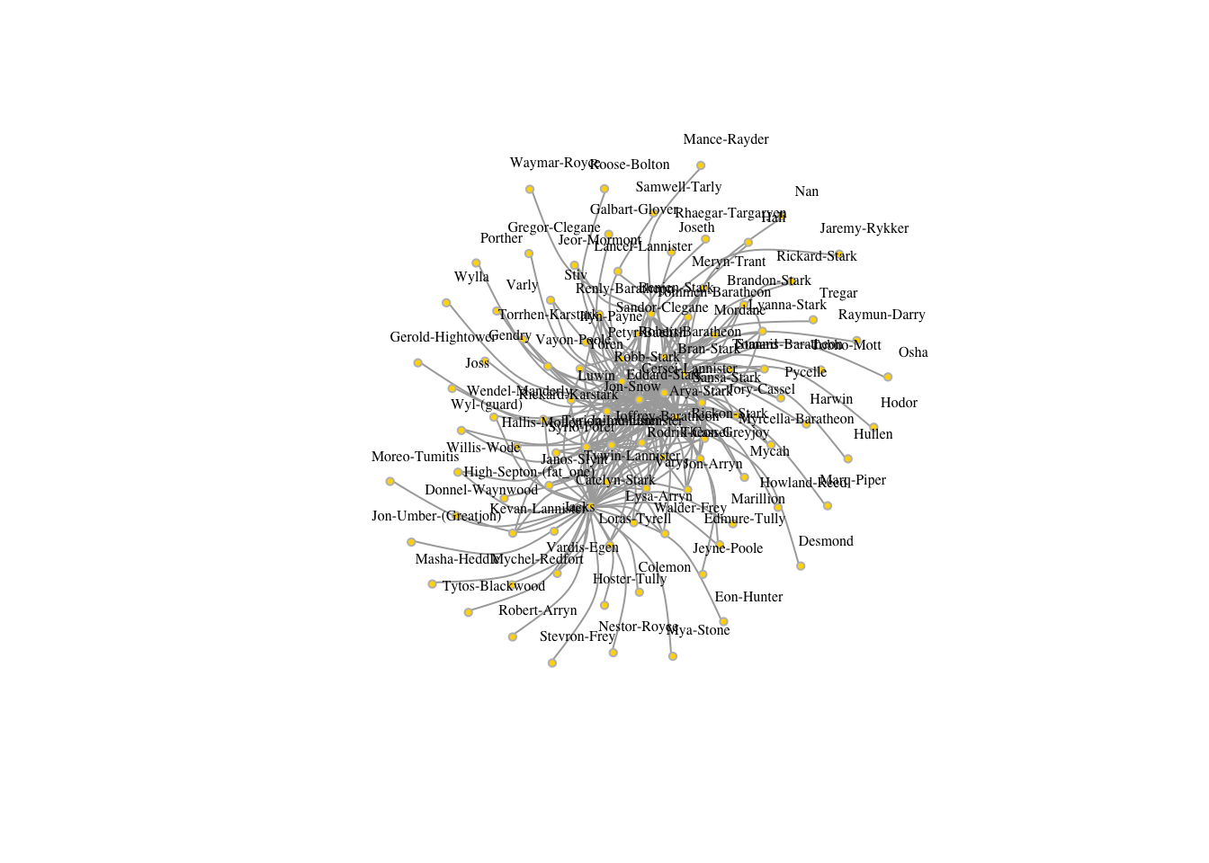

2.3.4.1.1 To make the graph look nicer

Node color: using family name
Node size: degree
Edge width: weight

## store the fullname
fullnames=V(got2)$name
fullnames[1:3]

## [1] "Arya-Stark"   "Benjen-Stark" "Bran-Stark"

#get family name
familynames=fullnames%>%str_split("-",simplify = TRUE)%>%.[,2]
familynames[familynames==""]="None"
familynames[familynames=="(guard)"]="None"
# add vertices attributes
V(got2)$familyname=familynames
V(got2)$fullname=fullnames
V(got2)$name=nameshort # first name

Set colors and legend.

pch: plotting symbols appearing in the legend
pt.bg: background color for point
cex: text size
pt.cex: point size
ncol: number of columns of the legend
bty: “o”– rectangle box; “n” – no box

vcol=V(got2)$familyname
vcol[(vcol!="Stark")&(vcol!="Lannister")]="gray50"
vcol[vcol=="Stark"]="tomato"
vcol[vcol=="Lannister"]="gold"
V(got2)$color=vcol
V(got2)$size=igraph::degree(got2)%>%log()*4
E(got2)$width=E(got2)$weight%>%log()/2
plot(got2, vertex.label.color="black", 
     vertex.label.cex=.5, vertex.label.dist=2, edge.curved=0.5,layout=layout_with_kk)
legend("right", legend = c("Stark","Lannister","Other"), pch=21,
       col=c("tomato","gold","gray50"), pt.bg=c("tomato","gold","gray50"), pt.cex=1, cex=.8, bty="n", ncol=1)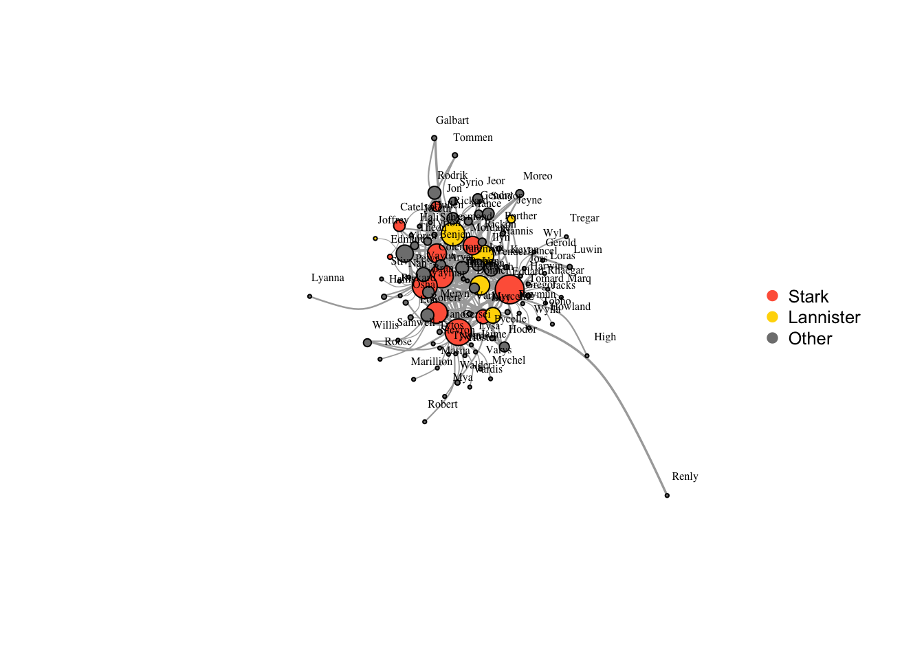

Plot only labels of the nodes

plot(got2, vertex.shape="none",vertex.label.color="black", 
     vertex.label.cex=.5, vertex.label.dist=2, edge.curved=0.5,layout=layout_with_kk)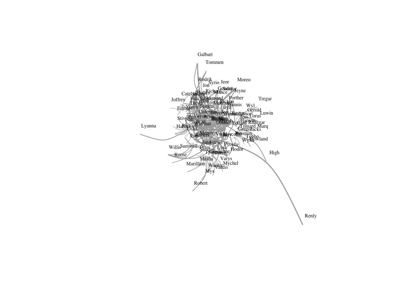

2.3.4.2 Layouts

Layouts from [Kateto tutorial](https://kateto.net/networks-r-igraph)

Figure 2.11: Layouts from Kateto tutorial

Force-directed layouts: suitable for general, small to medium sized graphs. (computational complexity; based on physical analogies)

layout_with_fr: Fruchterman-Reingold is one of the most used force-directed layout algorithms. Force-directed layouts try to get a nice-looking graph where edges are similar in length and cross each other as little as possible. As a result, nodes are evenly distributed through the chart area, and the layout is intuitive in that nodes which share more connections are closer to each other.
layout_with_kk: Another popular force-directed algorithm that produces nice results for connected graphs is Kamada Kawai.
layout_with_graphopt: …

For large graphs:

layout_with_lgl: The LGL algorithm is meant for large, connected graphs. Here you can also specify a root: a node that will be placed in the middle of the layout.
layout_with_drl:
layout_with_gfr:

layout_with_dh:simulated annealing algorithm by Davidson and Harel

#layout_with_dh
plot(got2, vertex.label.color="black", 
     vertex.label.cex=.5,vertex.label.dist=0.2, edge.curved=0.5,layout=layout_with_dh)
legend("right", legend = c("Stark","Lannister","Other"), pch=21,
       col=c("tomato","gold","gray50"), pt.bg=c("tomato","gold","gray50"), pt.cex=1, cex=.8, bty="n", ncol=1)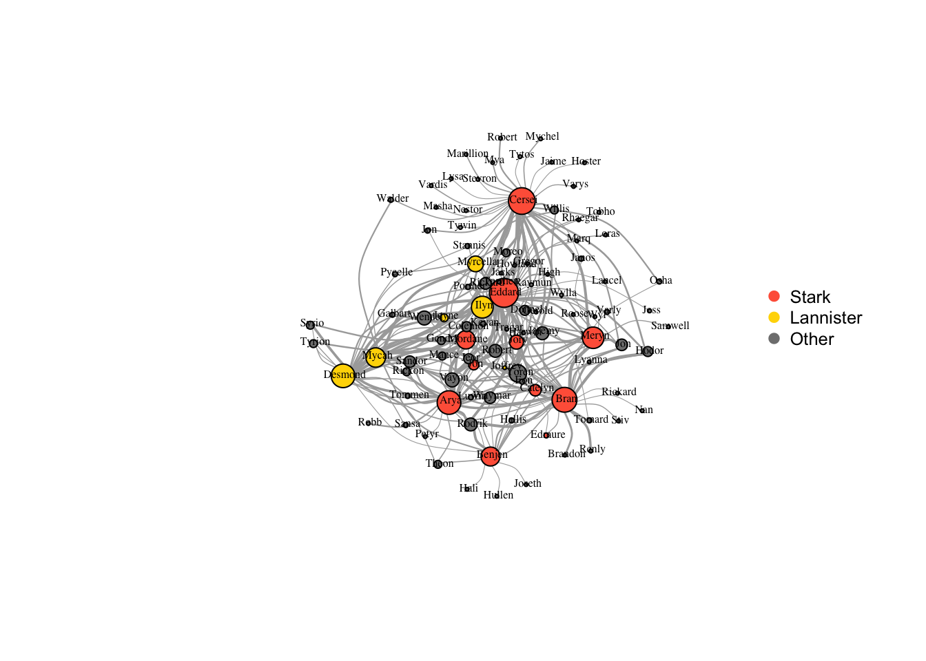

Selecting a layout automatically

connected and vcount<=100: kk
vcount<=1000:fr
else: drl

plot(got2, vertex.label.color="black", 
     vertex.label.cex=.5,vertex.label.dist=0.2, edge.curved=0.5,layout=layout.auto(got2))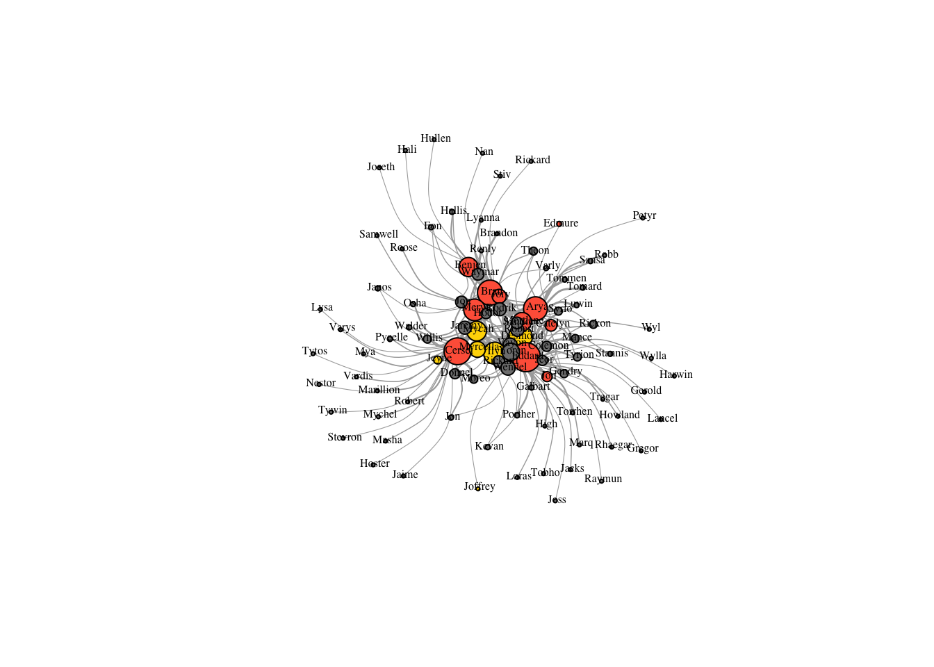

Without label and color the edge.

set.seed(2)
plot(got2, vertex.shape="none",vertex.label.color="black", 
     vertex.label.cex=.5,vertex.label.dist=0.2, edge.curved=0.5,layout=layout_with_dh)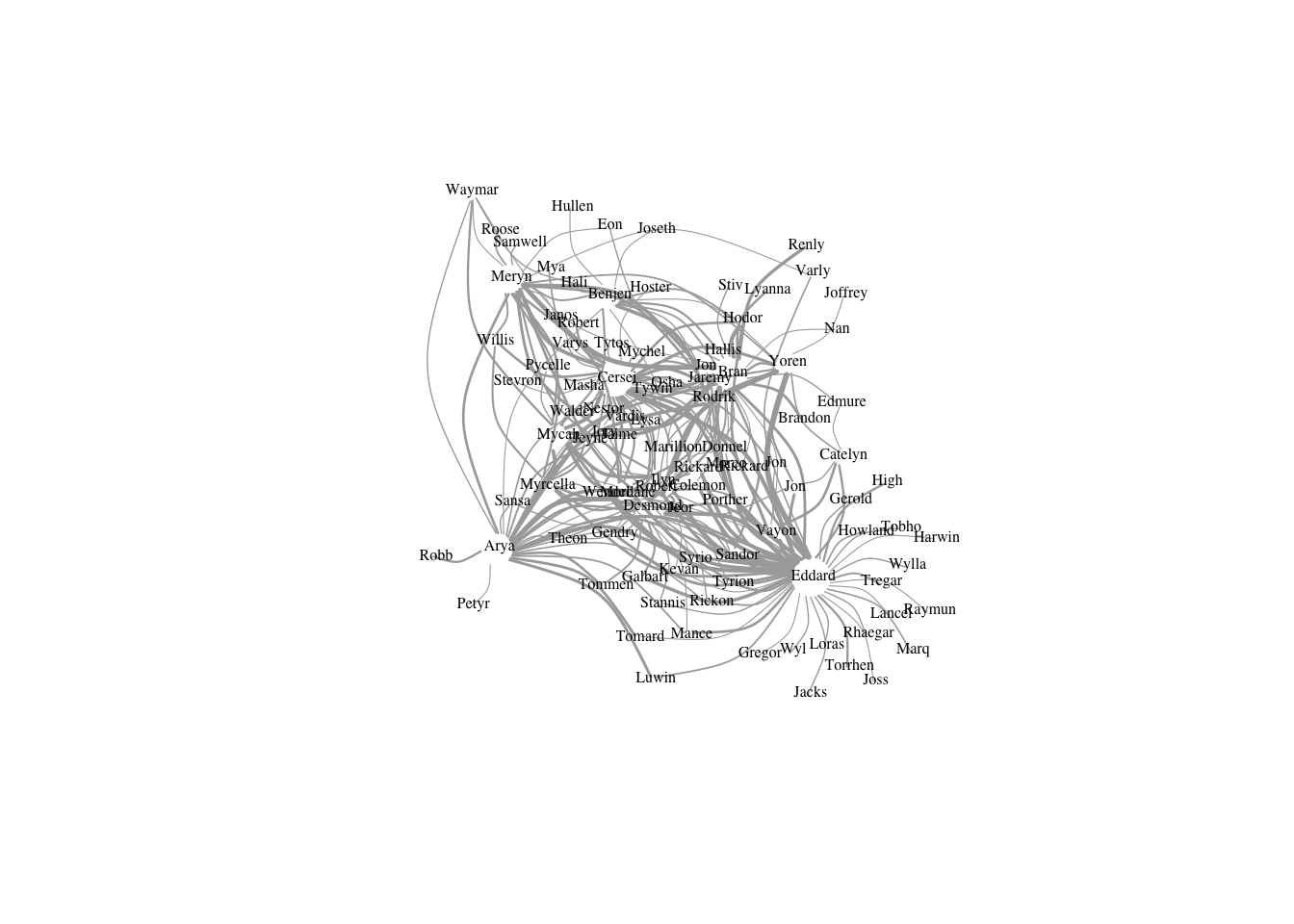

##color the edge
got2

## IGRAPH 21f2988 UNW- 99 238 -- 
## + attr: name (v/c), familyname (v/c), fullname (v/c), color (v/c),
## | size (v/n), Type (e/c), weight (e/n), book (e/n), source.family
## | (e/c), target.family (e/c), width (e/n)
## + edges from 21f2988 (vertex names):
##  [1] Arya--Benjen  Arya--Bran    Arya--Cersei  Arya--Desmond Arya--Petyr  
##  [6] Arya--Eddard  Arya--Rickon  Arya--Robb    Arya--Robert  Arya--Rodrik 
## [11] Arya--Sandor  Arya--Sansa   Arya--Syrio   Arya--Tomard  Arya--Tommen 
## [16] Arya--Vayon   Arya--Jory    Arya--Meryn   Arya--Yoren   Arya--Jaremy 
## [21] Arya--Jeor    Arya--Mordane Arya--Luwin   Arya--Mance   Arya--Theon  
## [26] Arya--Tyrion  Arya--Waymar 
## + ... omitted several edges

ecol=rep("gray50",ecount(got2))
ecol[E(got2)$source.family=="Stark"]="tomato"
ecol[E(got2)$source.family=="Lannister"]="gold"
ecol[(ecol=="tomato")&(E(got2)$target.family=="Lannister")&(!is.na(E(got2)$target.family))]="orange"
ecol[(ecol=="gold")&(E(got2)$target.family=="Stark")&(!is.na(E(got2)$target.family))]="orange"

set.seed(2)
plot(got2, vertex.shape="none",vertex.label.color="black", edge.color=ecol,
     vertex.label.cex=.5,vertex.label.dist=0.2, edge.curved=0.5,layout=layout_with_dh)
legend("right", legend = c("Stark","Lannister","Stark-Lannister","Other"),
       col=c("tomato","gold","orange","gray50"), lty=rep(1,4), cex=.8, bty="n", ncol=1)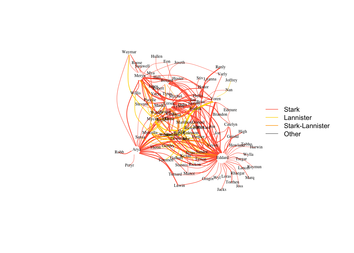

2.3.4.3 layout is not deterministic

Different runs will result in slightly different configurations. Saving the layout or set.seed allows us to get the exact same result multiple times, which can be helpful if you want to plot the time evolution of a graph, or different relationships – and want nodes to stay in the same place in multiple plots.

set.seed(1)
l=layout_with_dh(got2)
plot(got2, vertex.shape="none",vertex.label.color="black", 
     vertex.label.cex=.5,vertex.label.dist=0.2, edge.curved=0.5,layout=l)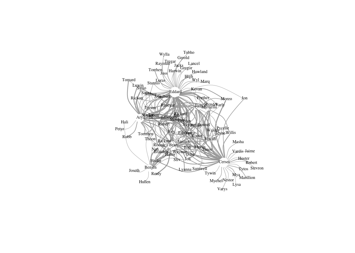

rescale

norm_coords
rescale=F
can use layout=l*2

l=layout_with_fr(got2)
l <- norm_coords(l, ymin=-1, ymax=1, xmin=-1, xmax=1) #default -- scaled
plot(got2, vertex.shape="none",vertex.label.color="black", 
     vertex.label.cex=.5,vertex.label.dist=0.2, edge.curved=0.5,layout=l,rescale=F)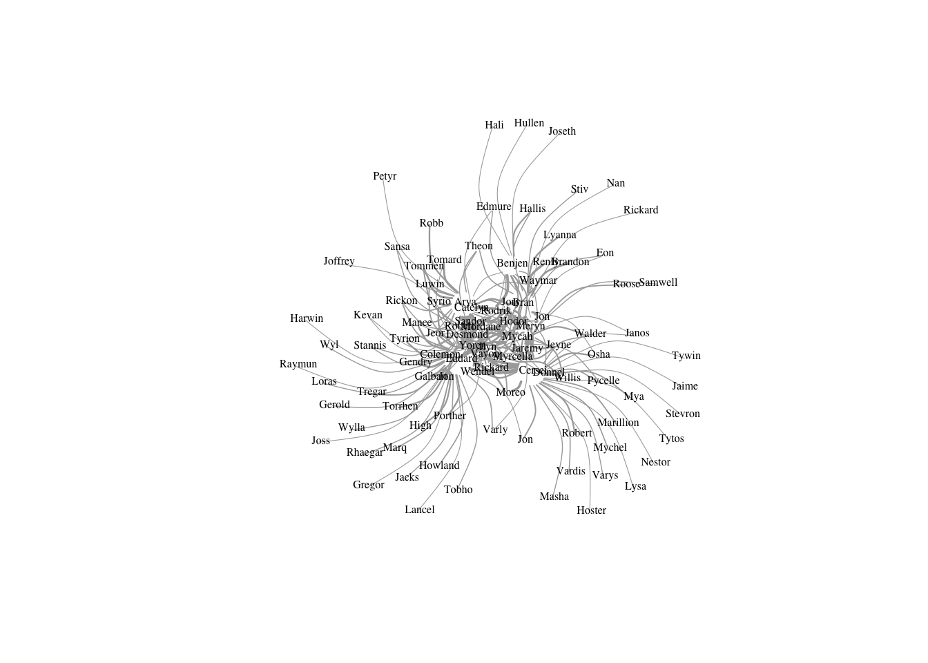

Will introduce interactive r packages next time.

par(mfrow=c(2,2), mar=c(0,0,0,0))
plot(got2, vertex.shape="none",vertex.label.color="black", 
     vertex.label.cex=.5,vertex.label.dist=0.2, edge.curved=0.5,layout=l*0.5,rescale=F)
plot(got2, vertex.shape="none",vertex.label.color="black", 
     vertex.label.cex=.5,vertex.label.dist=0.2, edge.curved=0.5,layout=l*0.8,rescale=F)
plot(got2, vertex.shape="none",vertex.label.color="black", 
     vertex.label.cex=.5,vertex.label.dist=0.2, edge.curved=0.5,layout=l*1,rescale=F) 
plot(got2, vertex.shape="none",vertex.label.color="black", 
     vertex.label.cex=.5,vertex.label.dist=0.2, edge.curved=0.5,layout=l*2,rescale=F)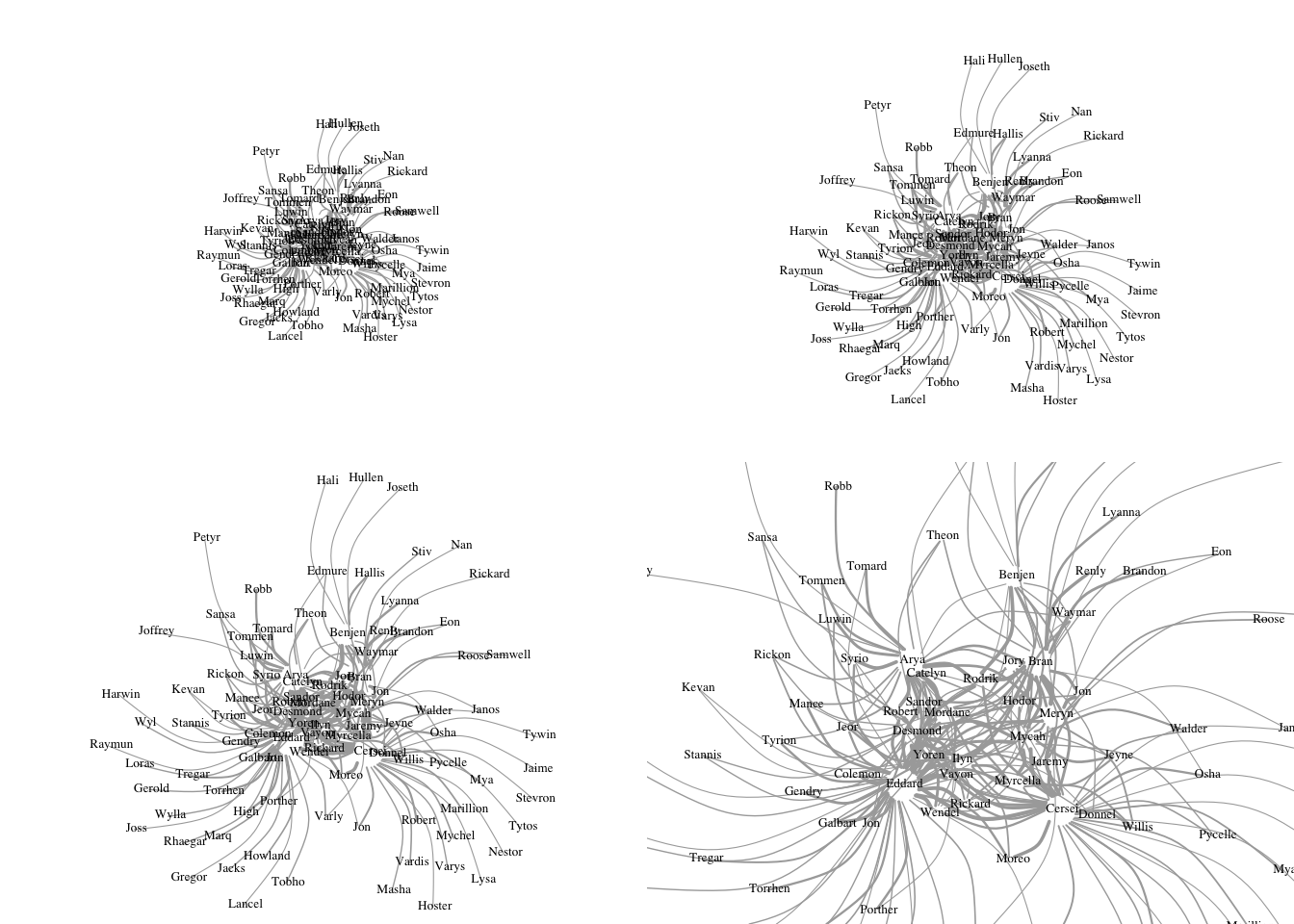

#dev.off()

2.3.5 Network and node descriptions

Density: edge_density
Degree: degree
centrality and centralization:
- centr_degree
- closeness, centr_clo
- eigen_centrality, centr_eigen
- betweenness, edge_betweenness, centr_betw
reciprocity,transitivity,diameter,…

2.3.5.1 Density

The proportion of present edges from all possible ties.

edge_density(got2, loops=F)

## [1] 0.04906205

ecount(got2)/(vcount(got2)*(vcount(got2)-1))*2 #for an undirected network

## [1] 0.04906205

2.3.5.2 Node degrees

‘degree’ has a mode of ‘in’ for in-degree, ‘out’ for out-degree, and ‘all’ or ‘total’ for total degree.

Notice the graph is undirected. So there is no difference under different parameter setting.

deg <- igraph::degree(got2, mode="all")
hist(deg, breaks=1:vcount(got2)-1, main="Histogram of node degree")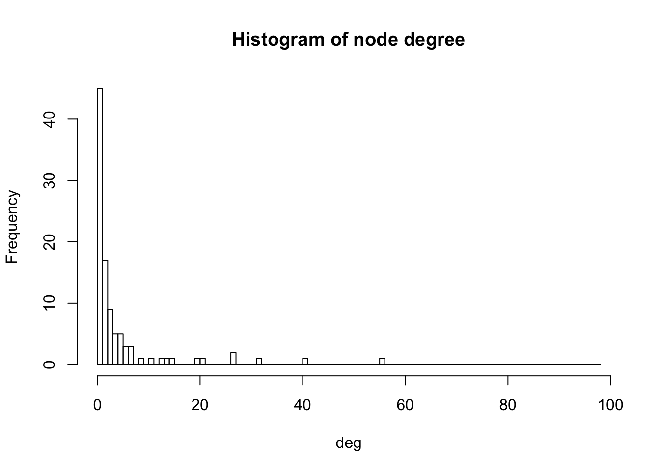

deg.dist <- degree_distribution(got2, cumulative=T, mode="all")
plot( x=0:max(deg), y=1-deg.dist, pch=19, cex=1.2, col="orange", 
      xlab="Degree", ylab="Cumulative Frequency")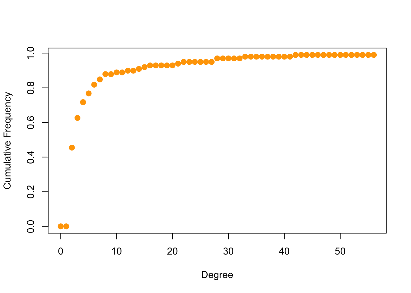

2.3.5.3 centrality and centralization

Who is the most important character?

Degree
Closeness
Eigenvector
Betweeness

Degree (number of ties).

Normalization should be the max degree the network can get

igraph::degree(got2, mode="in",loops = F)%>%sort(decreasing = TRUE)%>%.[1:5]

##  Eddard  Cersei    Bran    Arya Desmond 
##      56      41      32      27      27

#Notice this is undirected network, the choice of mode does not matter
centr_degree(got2, mode="in", normalized=T,loops = F)$res%>%sort(decreasing = TRUE)%>%.[1:5]

## [1] 56 41 32 27 27

centr_degree(got2, mode="all", normalized=T,loops = F)$res%>%sort(decreasing = TRUE)%>%.[1:5]

## [1] 56 41 32 27 27

#Pay attention to whether allowing self-loop or not
# Normalization may differ due to the setting
centr_degree(got2, mode="all", normalized=T,loops = F)$theoretical_max

## [1] 9506

centr_degree(got2, mode="in", normalized=T,loops = F)$theoretical_max

## [1] 9506

centr_degree(got2, mode="in", normalized=T,loops = T)$theoretical_max

## [1] 9702

Closeness (centrality based on distance to others in the graph) Inverse of the node’s average geodesic distance to others in the network

#whether to include weight or not
#If a graph has edge attribute weight, the weight will be automatically took into consideration
igraph::closeness(got2, mode="all", weights=NA) %>%sort(decreasing = TRUE)%>%.[1:5]

##      Eddard      Cersei        Bran        Arya     Desmond 
## 0.006993007 0.006329114 0.006097561 0.005882353 0.005847953

igraph::closeness(got2, mode="all")%>%sort(decreasing = TRUE)%>%.[1:5]

##       Eddard       Cersei       Donnel         Bran         Arya 
## 0.0010193680 0.0010111223 0.0010070493 0.0009990010 0.0009852217

centr_clo(got2, mode="all", normalized=T)$res %>%sort(decreasing = TRUE)%>%.[1:5]

## [1] 0.6853147 0.6202532 0.5975610 0.5764706 0.5730994

Eigenvector (centrality proportional to the sum of connection centralities) Values of the first eigenvector of the graph adjacency matrix

eigen_centrality(got2, directed=F, weights=NA)$vector%>%sort(decreasing = TRUE)%>%.[1:5]

##    Eddard    Cersei      Bran   Desmond      Arya 
## 1.0000000 0.8163499 0.7410532 0.7276696 0.6740883

eigen_centrality(got2, directed=F)$vector%>%sort(decreasing = TRUE)%>%.[1:5]

##    Eddard     Yoren   Desmond    Cersei     Vayon 
## 1.0000000 0.8538947 0.4281666 0.3352669 0.2441671

centr_eigen(got2, directed=F, normalized=T) $vector%>%sort(decreasing = TRUE)%>%.[1:5]

## [1] 1.0000000 0.8163499 0.7410532 0.7276696 0.6740883

Betweenness (centrality based on a broker position connecting others) (Number of geodesics that pass through the node or the edge)

igraph::betweenness(got2, directed=F, weights=NA)%>%sort(decreasing = TRUE)%>%.[1:5]

##    Eddard    Cersei      Bran      Arya     Meryn 
## 2155.2656 1554.1678  915.6561  510.5637  366.8074

igraph::betweenness(got2, directed=F)%>%sort(decreasing = TRUE)%>%.[1:5]

##    Eddard    Cersei      Bran    Benjen      Arya 
## 1835.5000 1483.2500 1024.8571  694.4762  689.5833

edge_betweenness(got2, directed=F, weights=NA)%>%sort(decreasing = TRUE)%>%.[1:5]

## [1] 426.4643 271.6982 198.3379 150.0371 133.8635

centr_betw(got2, directed=F, normalized=T)$res%>%sort(decreasing = TRUE)%>%.[1:5]

## [1] 2155.2656 1554.1678  915.6561  510.5637  366.8074

2.3.5.4 Other properties

transitivity
reciprocity
clustering coefficient
…

2.4 Paths, communitites and related visualization

2.4.1 Outline

R package igraph
- Paths
  - Paths, distances and diameter
  - Components
  - Transitivity and reciprocity
  - Max-flow and min-cut
- Communities
  - Pre-defined clusters
  - Different algorithms
- Visualization
  - Color the paths
  - Plotting clusters
  - Plotting dendrograms
  - Mark groups

2.4.2 Datasets

2.4.2.1 Load the datasets

data(USairports)
data(karate)

?USairports
?karate

2.4.2.2 Preprocess

USairports

## IGRAPH bf6202d DN-- 755 23473 -- US airports
## + attr: name (g/c), name (v/c), City (v/c), Position (v/c),
## | Carrier (e/c), Departures (e/n), Seats (e/n), Passengers (e/n),
## | Aircraft (e/n), Distance (e/n)
## + edges from bf6202d (vertex names):
##  [1] BGR->JFK BGR->JFK BOS->EWR ANC->JFK JFK->ANC LAS->LAX MIA->JFK
##  [8] EWR->ANC BJC->MIA MIA->BJC TEB->ANC JFK->LAX LAX->JFK LAX->SFO
## [15] AEX->LAS BFI->SBA ELM->PIT GEG->SUN ICT->PBI LAS->LAX LAS->PBI
## [22] LAS->SFO LAX->LAS PBI->AEX PBI->ICT PIT->VCT SFO->LAX VCT->DWH
## [29] IAD->JFK ABE->CLT ABE->HPN AGS->CLT AGS->CLT AVL->CLT AVL->CLT
## [36] AVP->CLT AVP->PHL BDL->CLT BHM->CLT BHM->CLT BNA->CLT BNA->CLT
## + ... omitted several edges

#should have no self-loop
sum(which_loop(USairports))

## [1] 53

USairports <- igraph::simplify(USairports, remove.loops = TRUE, remove.multiple = FALSE)
sum(which_loop(USairports))

## [1] 0

#different carrier and aircraft types leading to multiple graphs
USairports[["RDU","JFK",edges=TRUE]][[1]][[1:5]]

## + 5/23420 edges from 1fcdaeb (vertex names):
##       tail head tid hid                      Carrier Departures Seats
## 22271  RDU  JFK  74   4     Chautauqua Airlines Inc.         27  1350
## 20487  RDU  JFK  74   4 American Eagle Airlines Inc.         48  2112
## 20486  RDU  JFK  74   4 American Eagle Airlines Inc.         57  2109
## 14914  RDU  JFK  74   4                  Comair Inc.          1    76
## 14913  RDU  JFK  74   4                  Comair Inc.          5   250
##       Passengers Aircraft Distance
## 22271       1118      675      426
## 20487       1881      676      426
## 20486       1833      674      426
## 14914         68      638      426
## 14913        209      629      426

#simplify
air <- igraph::simplify(USairports, edge.attr.comb =list(Departures = "sum", Seats = "sum", Passengers = "sum",Distance="mean", "ignore"))
air

## IGRAPH 0073656 DN-- 755 8228 -- US airports
## + attr: name (g/c), name (v/c), City (v/c), Position (v/c),
## | Departures (e/n), Seats (e/n), Passengers (e/n), Distance (e/n)
## + edges from 0073656 (vertex names):
##  [1] BGR->BOS BGR->JFK BGR->MIA BGR->EWR BGR->DCA BGR->DTW BGR->LGA
##  [8] BGR->PHL BGR->PIE BGR->SFB BOS->BGR BOS->JFK BOS->LAS BOS->MIA
## [15] BOS->EWR BOS->LAX BOS->PBI BOS->PIT BOS->SFO BOS->IAD BOS->BDL
## [22] BOS->BUF BOS->BWI BOS->CAK BOS->CLE BOS->CLT BOS->CMH BOS->CVG
## [29] BOS->DCA BOS->DTW BOS->GSO BOS->IND BOS->LGA BOS->MDT BOS->MKE
## [36] BOS->MSP BOS->MSY BOS->MYR BOS->ORF BOS->PHF BOS->PHL BOS->RDU
## [43] BOS->RIC BOS->SRQ BOS->STL BOS->SYR BOS->ALB BOS->PVD BOS->ROC
## + ... omitted several edges

air[["RDU","JFK",edges=TRUE]]

## [[1]]
## + 1/8228 edge from 0073656 (vertex names):
## [1] RDU->JFK

2.4.3 Paths, distances and diameter

2.4.3.1 Paths

2.4.3.1.1 Select specific paths

Select specific paths

#select length 1 path
air[[from="RDU",to="BOS",edges=TRUE]]

## [[1]]
## + 1/8228 edge from 0073656 (vertex names):
## [1] RDU->BOS

# select >=1 paths
flight_rdu_bos=V(air)["RDU","JFK","BOS"]
E(air,path=flight_rdu_bos)

## + 2/8228 edges from 0073656 (vertex names):
## [1] RDU->JFK JFK->BOS

#another way
E(air)["RDU"%->%"JFK","JFK"%->%"BOS"]

## + 2/8228 edges from 0073656 (vertex names):
## [1] RDU->JFK JFK->BOS

2.4.3.1.2 Shortest paths

Many paths between edges. Direct flight or multiple steps.

Length of path: number of edges included in a path

shortest_paths: only one of the shortest paths

all_shortest_paths: all the shortest paths; nrgeo is the resultant vector of values from Djikstra’s algorithm which is used to find the shortest paths.

#arkansas airport-XNA
shortest_paths(air,from="RDU",to = "XNA",weights = E(air)$Distance)$vpath

## [[1]]
## + 3/755 vertices, named, from 0073656:
## [1] RDU CLT XNA

shortest_paths(air,from="RDU",to = "XNA",weights = NA)$vpath #one of the shortest path

## [[1]]
## + 3/755 vertices, named, from 0073656:
## [1] RDU LAS XNA

shortest_paths(air,from="RDU",to = "XNA",mode = "in",weights = NA)$vpath #to

## [[1]]
## + 3/755 vertices, named, from 0073656:
## [1] RDU BOS XNA

shortest_paths(air,from="RDU",to = "XNA",mode = "out",weights = NA)$vpath #from

## [[1]]
## + 3/755 vertices, named, from 0073656:
## [1] RDU LAS XNA

shortest_paths(air,from="RDU",to = "XNA",mode = "all",weights = NA)$vpath #undirected

## [[1]]
## + 3/755 vertices, named, from 0073656:
## [1] RDU BOS XNA

all_shortest_paths(air,from="RDU",to = "XNA",weight=NA)$res

## [[1]]
## + 3/755 vertices, named, from 0073656:
## [1] RDU MEM XNA
## 
## [[2]]
## + 3/755 vertices, named, from 0073656:
## [1] RDU DFW XNA
## 
## [[3]]
## + 3/755 vertices, named, from 0073656:
## [1] RDU DEN XNA
## 
## [[4]]
## + 3/755 vertices, named, from 0073656:
## [1] RDU ATL XNA
## 
## [[5]]
## + 3/755 vertices, named, from 0073656:
## [1] RDU ORD XNA
## 
## [[6]]
## + 3/755 vertices, named, from 0073656:
## [1] RDU IAH XNA
## 
## [[7]]
## + 3/755 vertices, named, from 0073656:
## [1] RDU MSP XNA
## 
## [[8]]
## + 3/755 vertices, named, from 0073656:
## [1] RDU LGA XNA
## 
## [[9]]
## + 3/755 vertices, named, from 0073656:
## [1] RDU DTW XNA
## 
## [[10]]
## + 3/755 vertices, named, from 0073656:
## [1] RDU CVG XNA
## 
## [[11]]
## + 3/755 vertices, named, from 0073656:
## [1] RDU CLT XNA
## 
## [[12]]
## + 3/755 vertices, named, from 0073656:
## [1] RDU EWR XNA
## 
## [[13]]
## + 3/755 vertices, named, from 0073656:
## [1] RDU LAS XNA

all_shortest_paths(air,from="RDU",to = "XNA",weights = E(air)$Distance)$res

## [[1]]
## + 3/755 vertices, named, from 0073656:
## [1] RDU CLT XNA

2.4.3.1.3 Color certain paths:

Color the path from Actor 33 to Mr Hi and set the width for the path.

path_vk=shortest_paths(karate,from="Actor 33", to="Mr Hi")$vpath[[1]]
ecol=rep("gray80",ecount(karate))
ecol[E(karate,path = path_vk)]="orange"
ew=rep(1,ecount(karate))
ew[E(karate,path = path_vk)]=3
plot(karate,edge.color=ecol,edge.width=ew)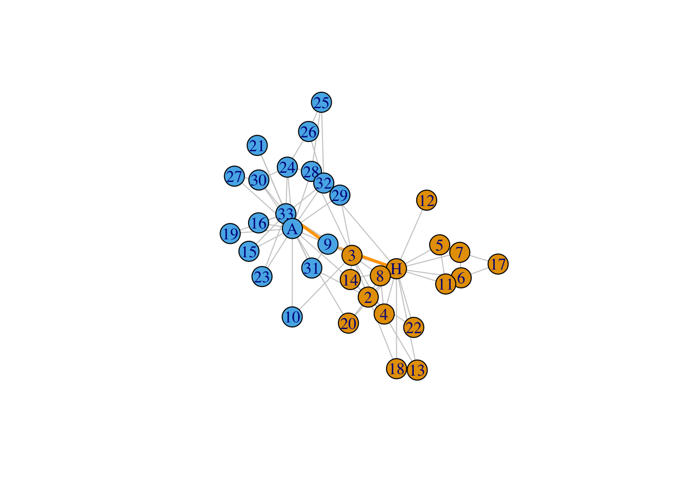

2.4.3.2 distance

Distance: length of shortest path

distance_table: The frequency of shortest path length between each pair of vertices.

distance_table(air)

## $res
## [1]   8228  94912 166335 163830  86263  15328   2793    291     27
## 
## $unconnected
## [1] 31263

# unconnected: the number of pairs for which the first vertex is not reachable from the second

distances

distances(air,"RDU","XNA",weights = NA) # not consider the weight

##     XNA
## RDU   2

distances(air,"RDU","XNA",weights =  E(air)$Distance) # specify the weight

##     XNA
## RDU 884

# how the function `distances` works
(shortest_paths(air,from="RDU",to = "XNA",weights = E(air)$Distance)$vpath[[1]])

## + 3/755 vertices, named, from 0073656:
## [1] RDU CLT XNA

E(air)["RDU"%->%"CLT","CLT"%->%"XNA"]$Distance%>%sum()

## [1] 884

#can return a distance matrix
distances(air,c("BOS","JFK","RDU","XNA"),c("BOS","JFK","RDU","XNA"),weights = E(air)$Distance,mode = "all") #undirected

##      BOS  JFK RDU  XNA
## BOS    0  187 612 1312
## JFK  187    0 426 1150
## RDU  612  426   0  884
## XNA 1312 1150 884    0

distances(air,c("BOS","JFK","RDU","XNA"),c("BOS","JFK","RDU","XNA"),weights = E(air)$Distance,mode = "in") #focus on to

##      BOS  JFK RDU  XNA
## BOS    0  187 612 1312
## JFK  187    0 426 1150
## RDU  612  426   0  884
## XNA 1313 1150 884    0

distances(air,c("BOS","JFK","RDU","XNA"),c("BOS","JFK","RDU","XNA"),weights = E(air)$Distance,mode = "out") #focus on from # tranpose of mode "in"

##      BOS  JFK RDU  XNA
## BOS    0  187 612 1313
## JFK  187    0 426 1150
## RDU  612  426   0  884
## XNA 1312 1150 884    0

mean_distance: average path length in a graph, by calculating the shortest paths between all pairs of vertices (both ways for directed graphs). does not consider edge weights currently and uses a breadth-first search.

# connected=TRUE
mean_distance(air,directed = TRUE)

## [1] 3.52743

# How the function works
freq=distance_table(air)$res/sum(distance_table(air)$res)
sum(freq*1:9)

## [1] 3.52743

#connected=FALSE
mean_distance(air,directed = TRUE,unconnected = FALSE)

## [1] 44.79658

#How the function works
freq=c(distance_table(air)$res,distance_table(air)$unconnected)/sum(c(distance_table(air)$res,distance_table(air)$unconnected))
sum(freq*c(1:9,vcount(air)))

## [1] 44.79658

2.4.3.3 Diameter

diameter: The largest distance of a graph. In the special case when some vertices are not reachable via a path from some others, returns the longest finite distance.

diameter(air)

## [1] 9

diameter(air,weights = E(air)$Distance)

## [1] 11257

diameter(air,directed = FALSE)

## [1] 8

#can also specify the unconnected=TRUE/FALSE

2.4.3.3.1 Get the nodes and edges of the airports in the longest path

#get the nodes
get_diameter(air,weights = E(air)$Distance)

## + 9/755 vertices, named, from 0073656:
## [1] VNY ORL OPF SDF STL SFO GUM SPN TIQ

dia_v=get_diameter(air,weights = E(air)$Distance)
# information of nodes
dia_v[[]]

## + 9/755 vertices, named, from 0073656:
##     name              City         Position
## 717  VNY      Van Nuys, CA N341235 W1182924
## 713  ORL       Orlando, FL N283244 W0811959
## 712  OPF         Miami, FL N255425 W0801642
## 78   SDF    Louisville, KY N381028 W0854410
## 80   STL     St. Louis, MO N384452 W0902136
## 18   SFO San Francisco, CA N373708 W1222230
## 178  GUM          Guam, TT N132900 E1444746
## 180  SPN        Saipan, TT N150708 E1454346
## 181  TIQ        Tinian, TT N145949 E1453705

# edges
E(air,path = dia_v)

## + 8/8228 edges from 0073656 (vertex names):
## [1] VNY->ORL ORL->OPF OPF->SDF SDF->STL STL->SFO SFO->GUM GUM->SPN SPN->TIQ

# info of edges
dia_e=E(air,path = dia_v)
dia_e[[]]

## + 8/8228 edges from 0073656 (vertex names):
##      tail head tid hid Departures Seats Passengers Distance
## 8184  VNY  ORL 717 713          1    12          4     2218
## 8178  ORL  OPF 713 712          1    12          4      193
## 8177  OPF  SDF 712  78          1    10          2      904
## 2696  SDF  STL  78  80         60  8220       5837      254
## 2735  STL  SFO  80  18         31  3852       2820     1736
## 804   SFO  GUM  18 178         26 10675       9951     5812
## 5350  GUM  SPN 178 180        164  7544       4554      129
## 5356  SPN  TIQ 180 181        283  1698       1576       11

## delete the flight with passengers <= 10 then recalculate the diameter

air_filt=delete_edges(air,E(air)[Passengers<=10])
get_diameter(air_filt,weights = E(air_filt)$Distance)

## + 8/755 vertices, named, from 5611041:
## [1] TIQ SPN GUM HNL LAX OKC NYL JQF

2.4.3.3.2 Color the paths along the diameter

First step is to select the edges along the path.

Then just change the edge attribute.

dia_vk=get_diameter(karate,directed = FALSE)
ecol=rep("gray80",ecount(karate))
ecol[E(karate,path = dia_vk)]="orange"
plot(karate,edge.color=ecol)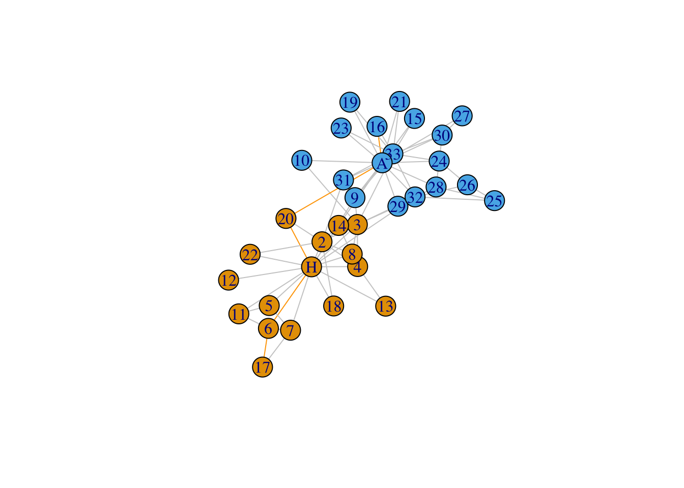

2.4.4 Components

2.4.4.1 Components

For an undirected graph,

Connected: if there is a path from any vertex to any other.

Unconnected: if not connected. An unconnected graph has multiple components.

Components: a maximal induced subgraph that is connected.

is_connected(air)

## [1] FALSE

count_components(air)

## [1] 6

#no:number of components
names(igraph::components(air))

## [1] "membership" "csize"      "no"

igraph::components(air)$csize

## [1] 745   2   2   3   2   1

igraph::components(air)$membership[igraph::components(air)$membership==6]

## DET 
##   6

# check whether RDU is in the largest component
subcomponent(air,"RDU") #not bad

## + 745/755 vertices, named, from 0073656:
##   [1] RDU BOS JFK LAS MIA EWR TEB PIT IAD BDL BNA BTR BWI CLE CLT CMH CVG
##  [18] DCA DTW GPT GSO ILM IND LEX LGA MDT MKE MSP PHL STL SYR TYS MHT PVD
##  [35] FLL MCO TPA IAH ORD CID MCI MSN SBN ATL DEN DFW MDW PHX RSW TUS ACY
##  [52] MEM SJU UTM SWO DAL ECP EVV LAN PIA FRG ISO BGR LAX PBI SFO BUF CAK
##  [69] MSY MYR ORF PHF RIC SRQ XNA ALB ROC SCE BHB PBG PQI AUS PDX SAN SEA
##  [86] SLC JAX STT SJC LGB PTK PGD IAG ACK LEB MVY PVC BMG AUG HYA RKD RUT
## [103] SLK ANC ABE AVP PWM SAV BTV SWF LWB CKB OKC HOU SAT SMF SNA BUR OAK
## [120] EGE BQN PSE FAR FWA FOE AEX GEG ICT BHM HPN LIT SDF MAF SHV MLI OMA
## [137] SGF TUL ABQ DSM GRR AMA LBB BOI HNL OGG ONT RNO COS ELP FAT GJT MFE
## [154] PSP BLI EUG ATW BIL BZN DLH FSD GRB GTF IDA MOT MSO BIS GFK RAP AZA
## + ... omitted several vertices

2.4.4.2 strongly connected and weakly connected

For a directed network,

weakly connected: its corresponding undirected network that ignored edge directions, is connected

strongly connected: if and only if it has a directed path from each vertex to all other vertices.

is_connected(air,mode = "weak")

## [1] FALSE

is_connected(air,mode = "strong")

## [1] FALSE

count_components(air,mode = "strong")

## [1] 30

igraph::components(air,mode = "strong")$membership%>%table()

## .
##   1   2   3   4   5   6   7   8   9  10  11  12  13  14  15  16  17  18 
##   1   1   1   1   1   1   1   1   1   1   2   1   2   1   1   2   1   1 
##  19  20  21  22  23  24  25  26  27  28  29  30 
##   1   1   1   1   1   1 723   1   1   1   1   1

# check whether RDU is in the largest component
"RDU"%in%(igraph::components(air,mode = "strong")$membership[igraph::components(air,mode = "strong")$membership==25]%>%names()) # not bad

## [1] TRUE

2.4.4.3 Transitivity and reciprocity

Network and node properties

2.4.4.4 Reciprocity

The proportion of reciprocated ties for a directed network

#number of reciprocity edges divided by number of edges
reciprocity(air)

## [1] 0.8762761

2*dyad_census(air)$mut/ecount(air)

## [1] 0.8762761

# number of mutual pairs divided by number of connected pairs
reciprocity(air,mode = "ratio")

## [1] 0.7797967

dyad_census(air)$mut/(dyad_census(air)$mut+dyad_census(air)$asym)

## [1] 0.7797967

#number of pairs
dyad_census(air)

## $mut
## [1] 3605
## 
## $asym
## [1] 1018
## 
## $null
## [1] 280012

2.4.4.5 transitivity

global: ratio of triangles to connected triples.

local: ratio of triangles to connected triples each vertex is part of.

transitivity(air,type = "global")

## [1] 0.3384609

transitivity(air,type = "local")[1:5]

## [1] 0.16842105 0.09683141 0.02803235 0.11144883 0.05888073

transitivity(air,vids = c("RDU","JFK"),type = "local") # specify multiple vertices

## [1] 0.4803279 0.3859649

#corresponds to different types of triples
triad_census(air)

##  [1] 68169544   712579  2380343     1445     1289     2465    15322
##  [8]    19171       91       39   114868      202      376      558
## [15]     6422    18671

?triad_census

2.4.4.6 maximum flows and minimum cuts

max flow How many passengers the US airport network can transport from a given airport to another one.

E(air)[["BOS"%->%"JFK"]]

## + 1/8228 edge from 0073656 (vertex names):
##    tail head tid hid Departures Seats Passengers Distance
## 12  BOS  JFK   2   4        491 39403      31426      187

# use seat to present the capacity.
max_flow(air,"BOS","JFK",capacity = E(air)$Seats)$value

## [1] 1177758

#capacity is for max_flow() function as default
E(air)$capacity=E(air)$Seats
max_flow(air,"BOS","JFK")$value

## [1] 1177758

min cut: the minimum number of edges, that disconnect a destination vertex from a departure vertex. In a weighted network with edge capacities the minimum cut calculates the total capacity needed to disconnect the vertex pair.

E(air)[["BOS"%->%"JFK"]]

## + 1/8228 edge from 0073656 (vertex names):
##    tail head tid hid Departures Seats Passengers Distance capacity
## 12  BOS  JFK   2   4        491 39403      31426      187    39403

# use seat to present the capacity.
min_cut(air,"BOS","JFK",capacity = E(air)$Seats)

## [1] 1177758

#capacity is for max_flow() function as default
E(air)$capacity=E(air)$Seats
min_cut(air,"BOS","JFK")

## [1] 1177758

max-flow min-cut theorem: the minimum cut in a graph from a source vertex to a target vertex always equals the maximum flow between the same vertices.

min_cut(air,"BOS","JFK",capacity = E(air)$Seats)

## [1] 1177758

max_flow(air,"BOS","JFK",capacity = E(air)$Seats)$value

## [1] 1177758

2.4.5 Community

2.4.5.1 Make clusters

You can speicfy the cluster as you want.

data("karate")

#ground truth
V(karate)$Faction

##  [1] 1 1 1 1 1 1 1 1 2 2 1 1 1 1 2 2 1 1 2 1 2 1 2 2 2 2 2 2 2 2 2 2 2 2

ground_truth=make_clusters(karate,V(karate)$Faction)
ground_truth

## IGRAPH clustering unknown, groups: 2, mod: 0.37
## + groups:
##   $`1`
##    [1]  1  2  3  4  5  6  7  8 11 12 13 14 17 18 20 22
##   
##   $`2`
##    [1]  9 10 15 16 19 21 23 24 25 26 27 28 29 30 31 32 33 34
##

#cluster by the distance
dist_memb=karate %>%
distances(v = c("John A", "Mr Hi")) %>% 
  apply(2, which.min) %>%
make_clusters(graph = karate)

2.4.5.2 Community detection

Different algorithm for community detection (clustering)

2.4.5.3 Girvan-Newman algorithm

Girvan-Newman algorithm (edge betweenness method): the number of shortest paths passing through an intra-community edge should be low while inter-community edges are likely to act as bottlenecks that participate in many shortest paths between vertices of different communities.

dendrogram <- cluster_edge_betweenness(karate)

## Warning in cluster_edge_betweenness(karate): At community.c:460 :Membership
## vector will be selected based on the lowest modularity score.

## Warning in cluster_edge_betweenness(karate): At community.c:467 :Modularity
## calculation with weighted edge betweenness community detection might not
## make sense -- modularity treats edge weights as similarities while edge
## betwenness treats them as distances

dendrogram

## IGRAPH clustering edge betweenness, groups: 6, mod: 0.35
## + groups:
##   $`1`
##   [1] "Mr Hi"    "Actor 2"  "Actor 4"  "Actor 8"  "Actor 12" "Actor 13"
##   [7] "Actor 18" "Actor 20" "Actor 22"
##   
##   $`2`
##   [1] "Actor 3"  "Actor 10" "Actor 14" "Actor 29"
##   
##   $`3`
##   [1] "Actor 5"  "Actor 6"  "Actor 7"  "Actor 11" "Actor 17"
##   
##   + ... omitted several groups/vertices

plot_dendrogram(dendrogram) # for hierarchical structure

membership(dendrogram) # best cut in terms of modularity

##    Mr Hi  Actor 2  Actor 3  Actor 4  Actor 5  Actor 6  Actor 7  Actor 8 
##        1        1        2        1        3        3        3        1 
##  Actor 9 Actor 10 Actor 11 Actor 12 Actor 13 Actor 14 Actor 15 Actor 16 
##        4        2        3        1        1        2        4        4 
## Actor 17 Actor 18 Actor 19 Actor 20 Actor 21 Actor 22 Actor 23 Actor 24 
##        3        1        4        1        4        1        4        5 
## Actor 25 Actor 26 Actor 27 Actor 28 Actor 29 Actor 30 Actor 31 Actor 32 
##        5        5        6        5        2        6        4        4 
## Actor 33   John A 
##        4        4

cut_at(dendrogram,no = 2) # cut into two groups

##  [1] 2 2 1 2 2 2 2 2 1 1 2 2 2 1 1 1 2 2 1 2 1 2 1 1 1 1 1 1 1 1 1 1 1 1

V(karate)[Faction == 1]$shape <- "circle"
V(karate)[Faction == 2]$shape <- "square"
set.seed(1)
plot(dendrogram,karate)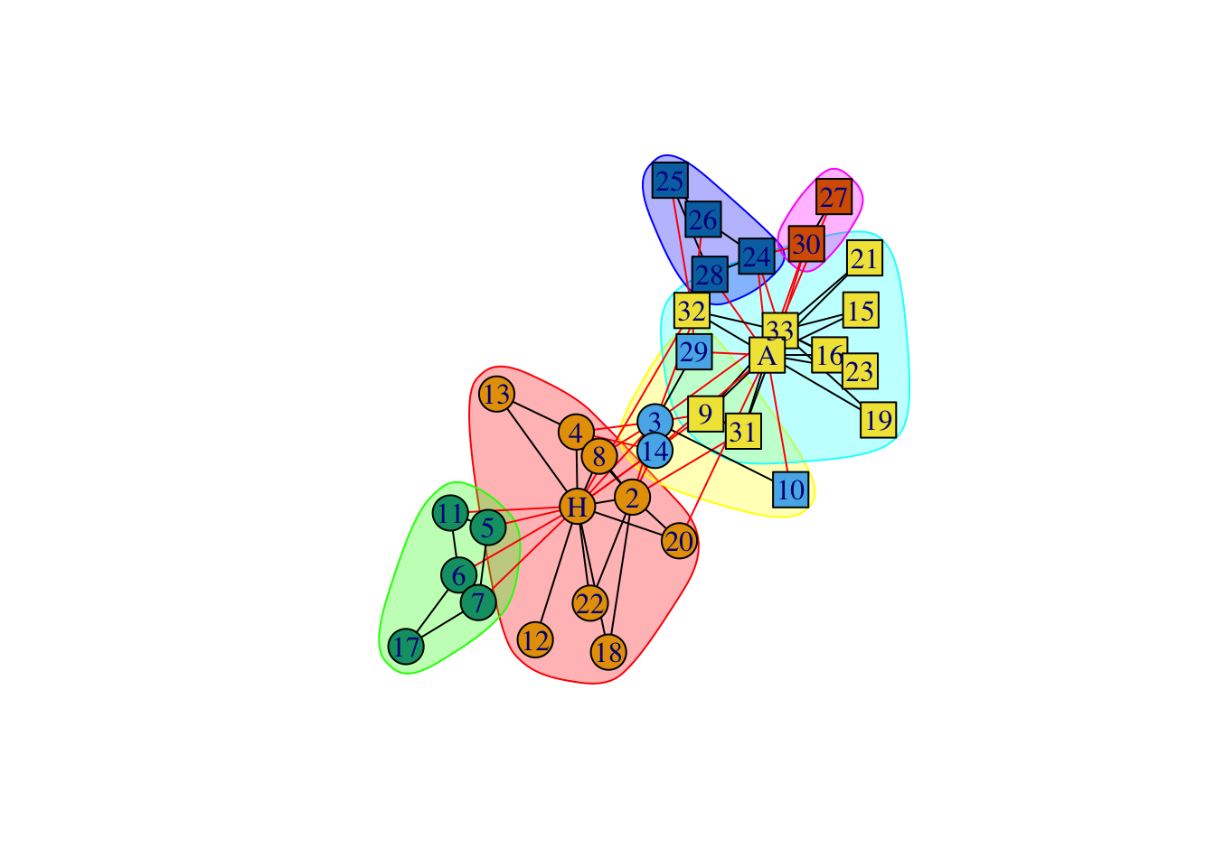

2.4.5.4 Exact modularity maximization

Exact modularity maximization: optimization problem to maximum the modularity

cluster_optimal() is not available for the underlying package is removed from CRAN
For large graph, apply cluster_fast_greedy()

#optimal=cluster_optimal(karate)
#set.seed(1)
#plot(optimal,karate)
optimal_lg=cluster_fast_greedy(karate)
set.seed(1)
plot(optimal_lg,karate)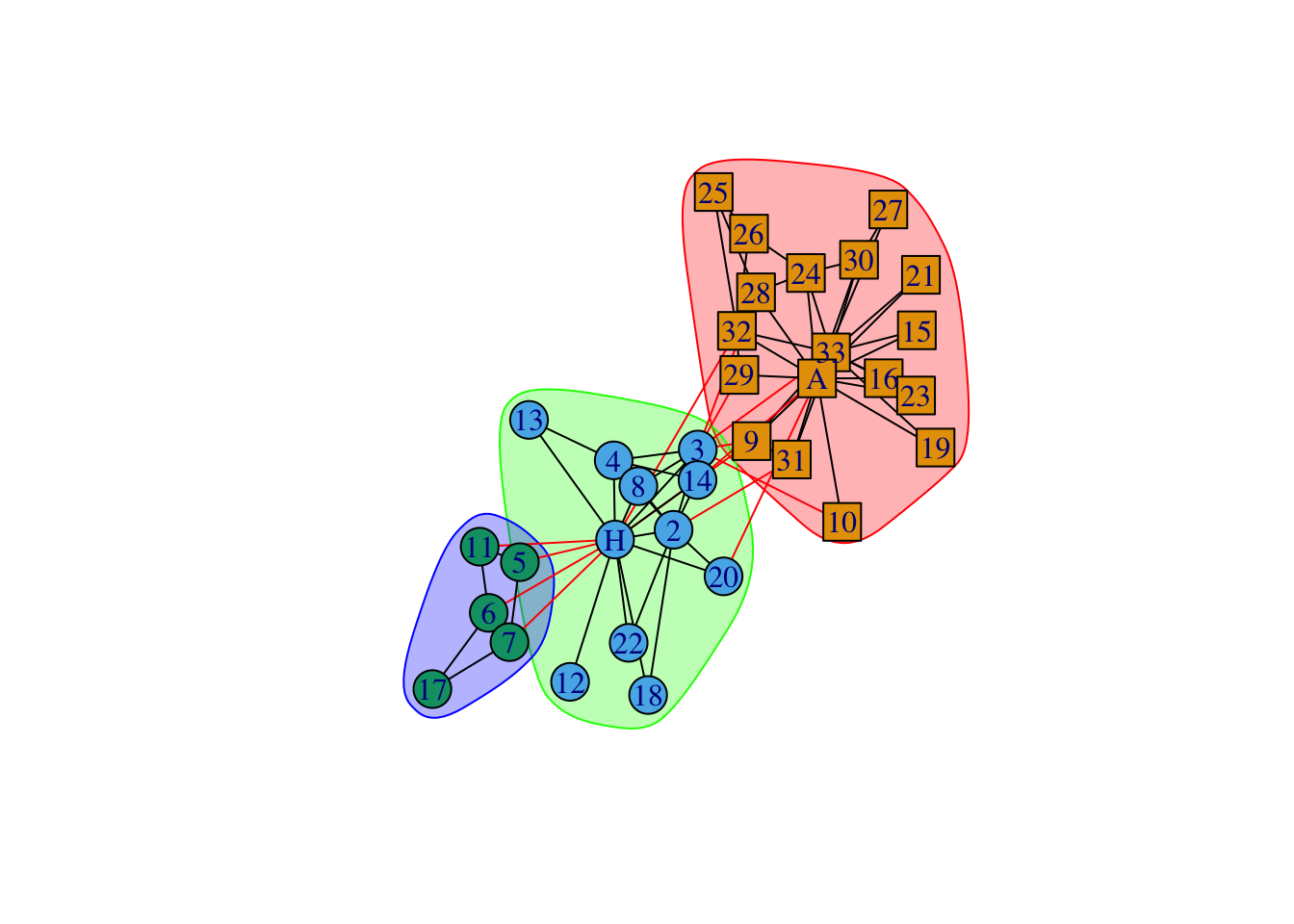

2.4.5.5 Leading eigenvector

eigen=cluster_leading_eigen(karate)
set.seed(1)
plot(eigen,karate)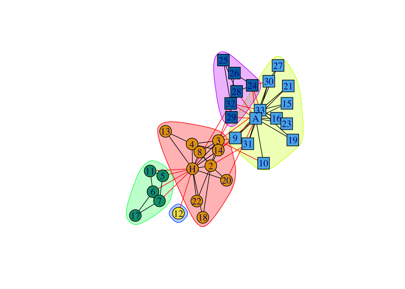

clusters <- cluster_leading_eigen(karate, steps = 1) #at most two cluster

2.4.5.6 Label propagation algorithm:

The algorithm terminates when it holds for each node that it belongs to a community to which a maximum number of its neighbors also belong.

fixed: TRUE-label will not change.
initial: initial point.

#non-negative values: different labels; negative values: no labels
initial=rep(-1,vcount(karate))
fixed=rep(FALSE,vcount(karate))
#need to have names
names(initial)=names(fixed)=V(karate)$name 
initial['Mr Hi']=1
initial['John A']=2
fixed['Mr Hi']=fixed['John A']=TRUE
lab=cluster_label_prop(karate,initial = initial,fixed = fixed)
set.seed(1)
plot(lab,karate)

set.seed(1)
plot(ground_truth,karate)

2.4.5.7 Other algorithms:

cluster_spinglass

…

2.4.6 Visualization

2.4.6.1 Visulization

color the paths
plotting clusters
plotting dendrograms
marked several grouping vertices

plot support igraph and other igraph objects such as vertexclustering, vertexdendrogram, …

2.4.6.2 Plotting clusters

plot(vertexdendrogram,igraph)

set.seed(1)
plot(ground_truth,karate)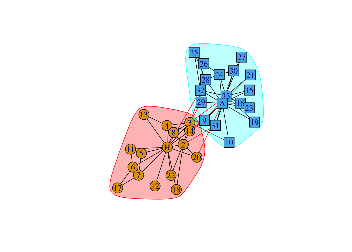

2.4.6.3 Plotting dendrograms

plot_dendrogram(vertexdendrogram)

Not flexible enough. Try ggdendrogram() in ggplot2 package.

set.seed(1)
plot_dendrogram(dendrogram)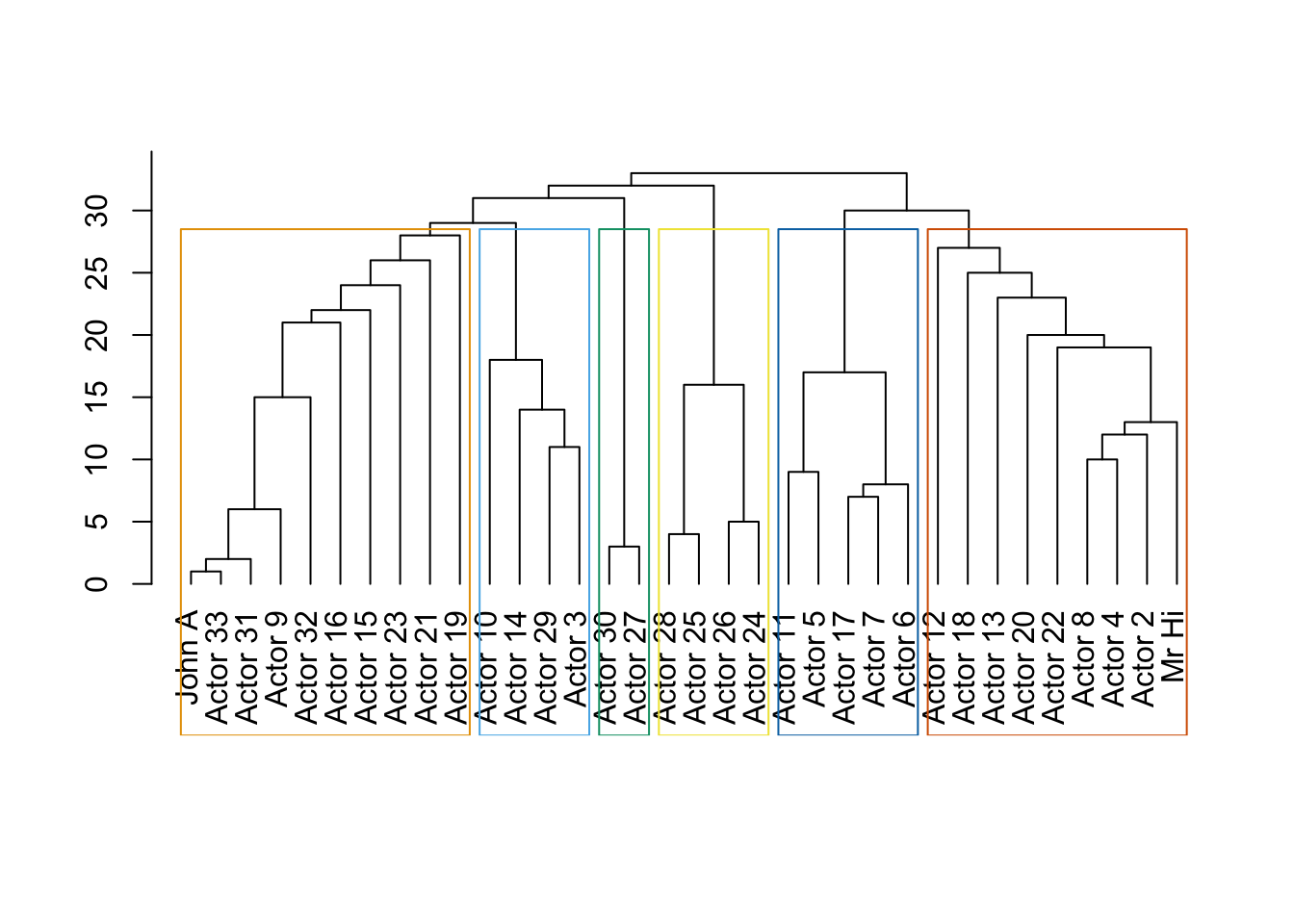

#labels at the same height: hang=-1
#cex: size of labels
plot_dendrogram(dendrogram,hang = -1, cex = 0.6)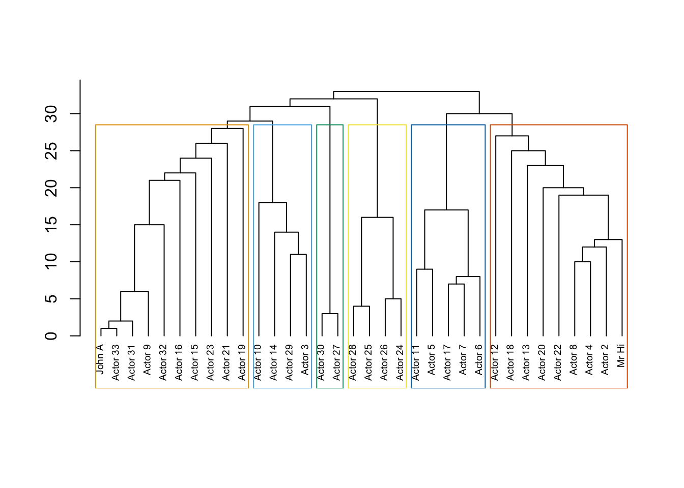

2.4.6.4 marked groups

plot:

mark.group: list
mark.col: vector
mark.border: vector
mark.shape: vector (smoothness of the border, range from -1 to 1)
mark.expand: vector (size of the border)

ls=list(`1`=ground_truth[[1]],`2`=ground_truth[[2]])
ls

## $`1`
##  [1]  1  2  3  4  5  6  7  8 11 12 13 14 17 18 20 22
## 
## $`2`
##  [1]  9 10 15 16 19 21 23 24 25 26 27 28 29 30 31 32 33 34

# other pars can be set as default
set.seed(1)
plot(karate,mark.groups = ls)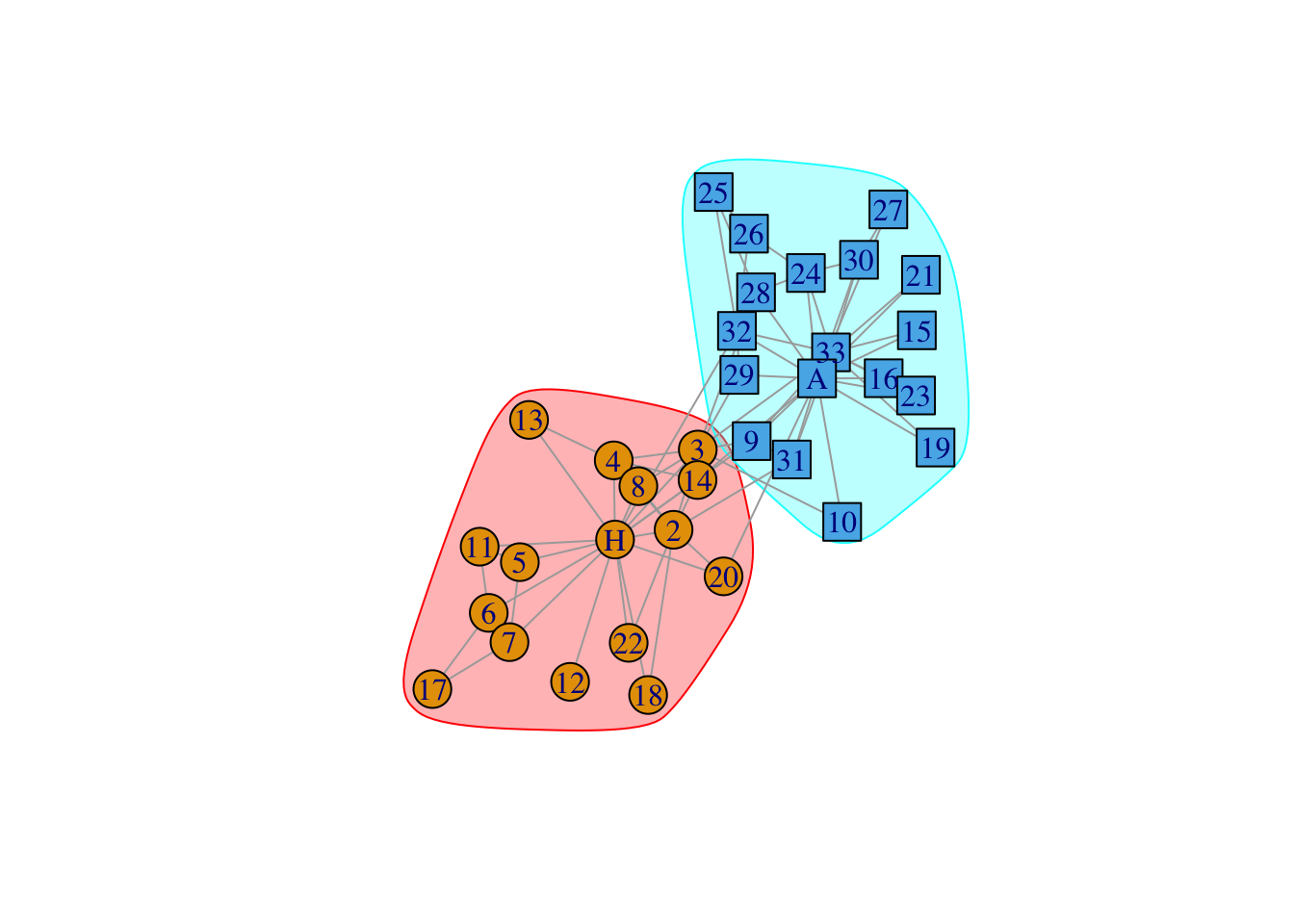

set.seed(1)
plot(karate,mark.groups = ls,mark.col = c("lightblue","yellow"),mark.border = rainbow(length(ls),alpha=1),mark.shape=c(-0.5,1),mark.expand = 1:2)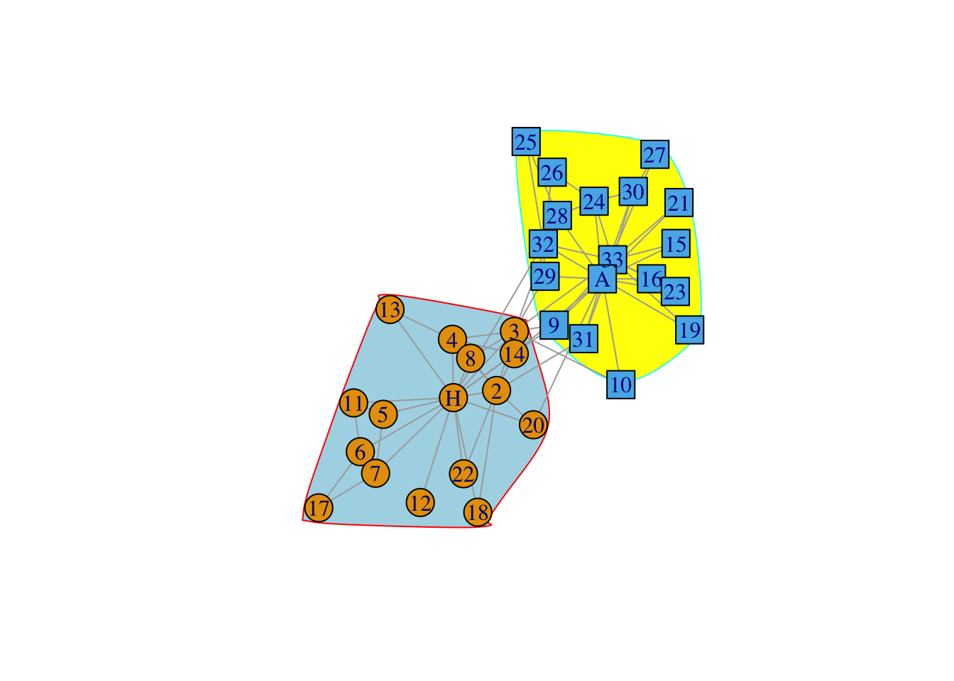

2.5 More about `igraph`

Epidemics on networks: compartmental models on netwoks
Spectral embeddings: community detection
Change-point detection in temporal graphs
CLustering multiple graphs
Cliques and graphlets
Graphons
Graph matching

Chapter 2 igraph package