Chapter 5 Advanced Network Visualization
5.1 Introduction
5.1.1 Outline
- Visualization for static network:
- Graph: hairball plot
- Matrix:
heatmapin R basic package;geom_tilein pkgggplot2
- Other static networks:
- Two-mode networks (node-specific attribute)
- Multiple networks (edge-specific attribute)
- … (
ggtree,ggalluvial, etc.)
ggplot2version for network visualization:- Comparison between
ggnet2,geomnet,ggnetwork - Extension to interactive (
plotly) , dynamic network (ggnetwork)
- Comparison between
- Other interactive network visualizations:
visNetwork(good documentation)networkD3threejsggigraph
- Visualization for dynamic networks
- Snapshots for the evolving networks:
ggnetwork(common) - Animation for the evolving networks:
ggplot2+gganimate ndtvpkg (good documentation)
- Snapshots for the evolving networks:
5.1.2 Available R packages and tutorial
ggplot2 version for network visualization
ggnet2: https://briatte.github.io/ggnet/geomnet: https://github.com/sctyner/geomnet https://cran.r-project.org/web/packages/geomnet/geomnet.pdfggnetwork: https://briatte.github.io/ggnetwork/
Comparison among the three R packages: https://journal.r-project.org/archive/2017/RJ-2017-023/RJ-2017-023.pdf
Interactive network visualization
visNetworkhttps://datastorm-open.github.io/visNetwork/ggigraphhttp://davidgohel.github.io/ggiraph/index.htmlnetworkD3http://christophergandrud.github.io/networkD3/threejshttp://bwlewis.github.io/rthreejs/graphjs.html https://bwlewis.github.io/rthreejs/
Dynamic network
ndtv- Official website: https://cran.r-project.org/web/packages/ndtv/vignettes/ndtv.pdf
- Nice tutorial: http://statnet.csde.washington.edu/workshops/SUNBELT/current/ndtv/ndtv_workshop.html#understanding-how-networkdynamic-works http://kateto.net/network-visualization http://statnet.csde.washington.edu/workshops/SUNBELT/current/ndtv/ndtv-d3_vignette.html
gganimatehttps://gganimate.com/ (ggplot2+gganimate)
Tutorial:
5.1.3 References
All code comes from the following websites with modifications:
5.2 Preparation
library(igraph)
library(igraphdata)
library(dplyr)
library(ggplot2)
data(karate)
5.3 Visualization for static network
5.3.1 Hairball plot
dia_vk=get_diameter(karate,directed = FALSE)
ecol=rep("gray80",ecount(karate))
ecol[E(karate,path = dia_vk)]="orange"
ew=rep(1,ecount(karate))
ew[E(karate,path = dia_vk)]=3
ls=list(`1`=which(V(karate)$Faction==1),`2`=which(V(karate)$Faction==2))
set.seed(1)
plot(karate,edge.color=ecol,edge.width=ew,mark.groups = ls)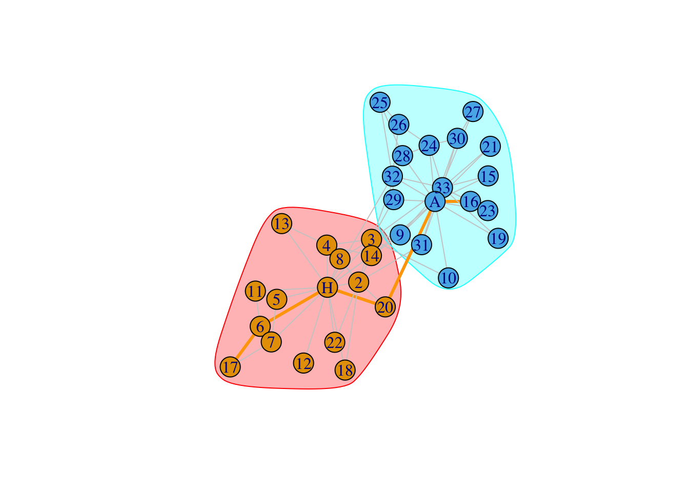
#,vertex.size=log(degree(karate))*7+15.3.2 Heatmap
karate.mat=get.adjacency(karate,sparse = FALSE)
heatmap(karate.mat[,34:1],Rowv = NA, Colv = NA,scale="none")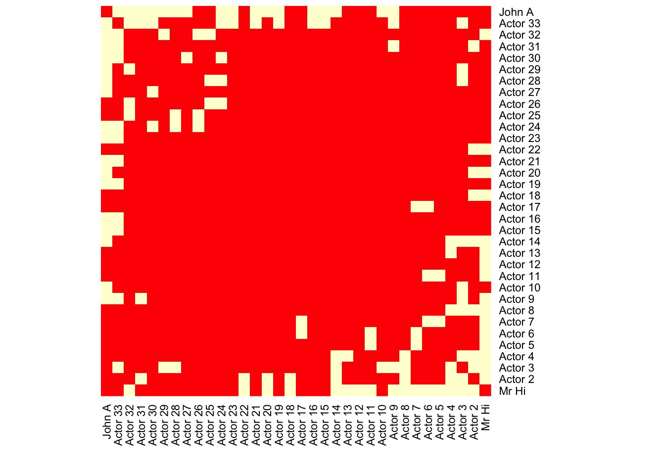
# By default, Rowv and Colv will provide us the dendrogram
#scale=c("row","column","none") -- normalize the values
heatmap(karate.mat[,34:1])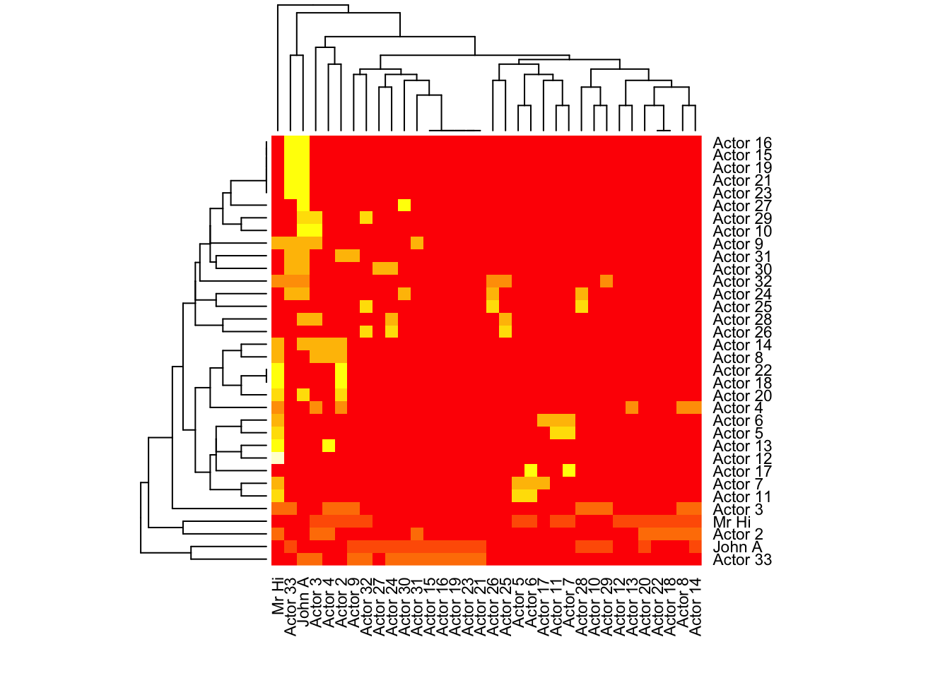
?heatmapUsing geom_tile in R package ggplot2:
# Change to long format. -- edgelist but including all the 0s
longData=reshape2::melt(karate.mat)
  longData_all=as_tibble(longData)
  longData_all1=longData_all%>%mutate(Var1=forcats::fct_rev(Var1))

# using geom_tile
ggplot(longData_all1, aes(x = Var2, y = Var1)) +
  geom_tile(aes(fill=value)) +
  scale_fill_gradient(low="white", high="#333333",na.value = "red") +
  theme_bw()+ggtitle("")+xlab("")+ylab("")+ #set clean background and no titles
  guides(fill = guide_colourbar(barheight = 12))+ # can set the length of colour bar
  theme(axis.text.x = element_text(angle = 90, hjust = 1))+
  coord_fixed() # fix to square coordinator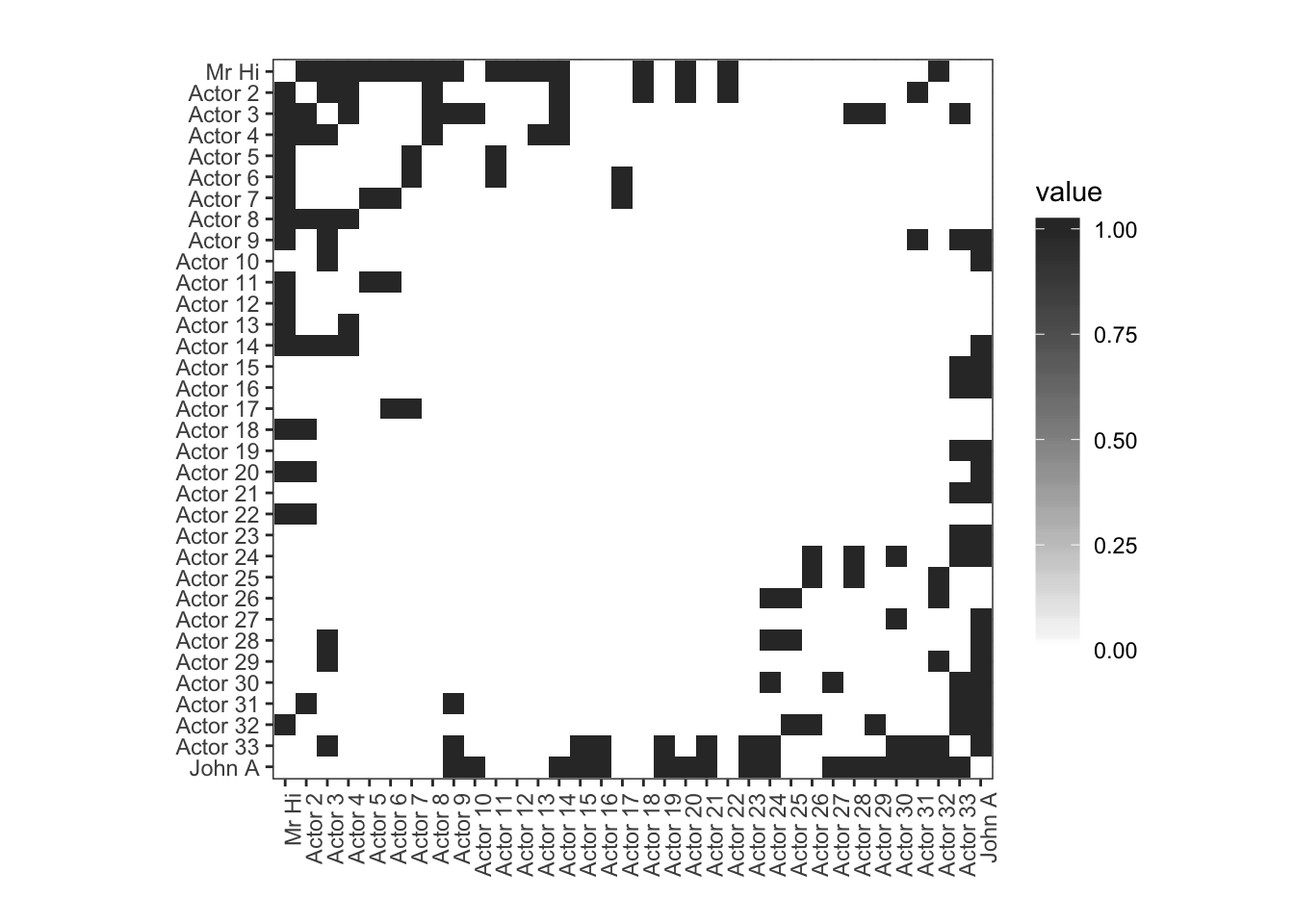
5.4 Other static networks
- Two-mode networks (different shape, color)
- Multiple networks (different color of edges, facets)
ggtreeggalluvial
5.4.1 Two-mode network
graph_from_incidence_matrix: add a vertex attribute called “type”- can use different node-specific plotting parameter (shape,color,label) to indicate the type
- has it own layout,
layout_as_bipartite
set.seed(1)
twomode.mat=matrix(sample(c(0,1),9,replace = TRUE),nrow = 3)
rownames(twomode.mat)=c("A","B","C")
colnames(twomode.mat)=1:3
twomode.mat
## 1 2 3
## A 0 1 1
## B 0 0 1
## C 1 1 1twomode.net=graph_from_incidence_matrix(twomode.mat)
plot(twomode.net)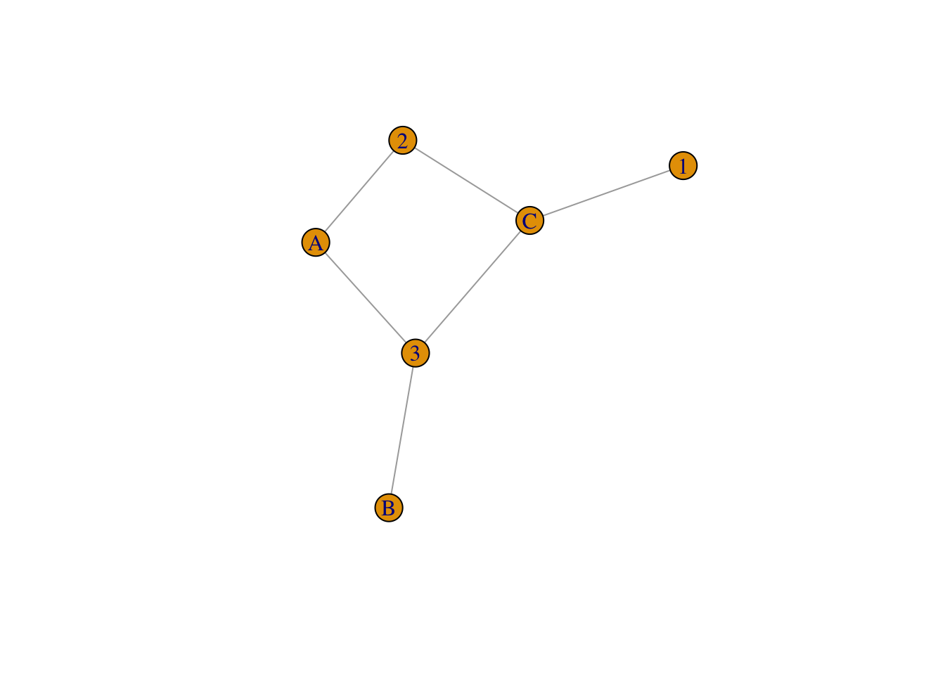
vertex_attr_names(twomode.net)## [1] "type" "name"V(twomode.net)$type## [1] FALSE FALSE FALSE TRUE TRUE TRUEV(twomode.net)$color <- c("blue", "orange")[V(twomode.net)$type+1]
V(twomode.net)$shape <- c("square", "circle")[V(twomode.net)$type+1]
plot(twomode.net,vertex.label.color="white")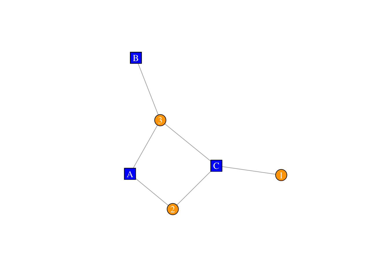
plot(twomode.net,vertex.label.color="white",layout=layout_as_bipartite)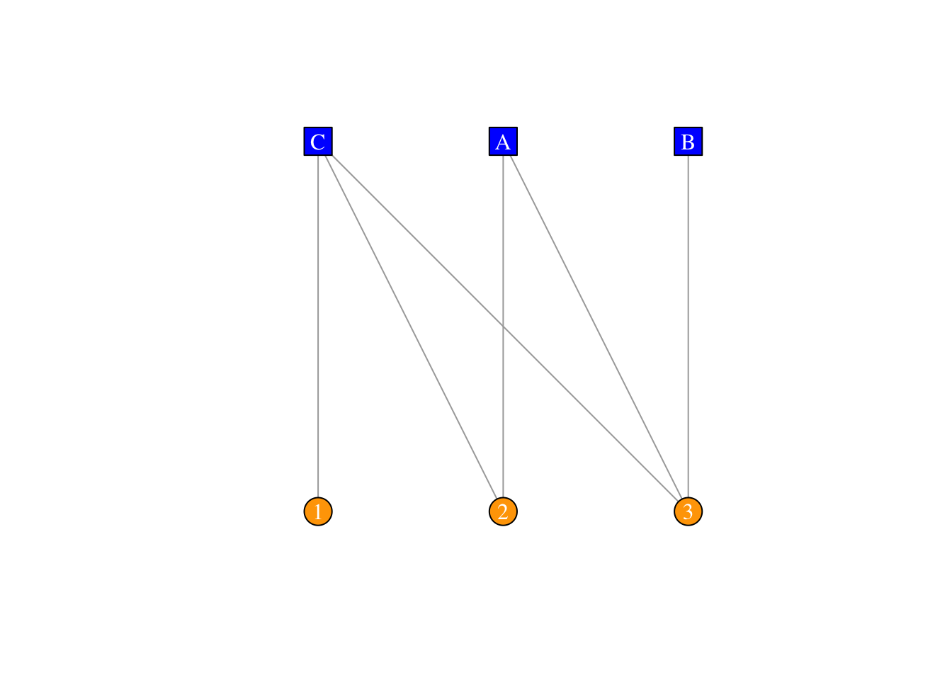
5.4.2 Multiple neworks
- can use different edge-specific plotting parameters (color,linetype) to indicate the type
- simplify the network by types.
- can use different facet to present different networks with fixing layout (using
ggnetworkwill be more convenient)
data(enron)
subenron=induced_subgraph(enron,V(enron)[1:30])
subenron
## IGRAPH af878f6 D--- 30 2133 -- Enron email network
## + attr: LDC_names (g/c), LDC_desc (g/c), name (g/c), Citation
## | (g/c), Email (v/c), Name (v/c), Note (v/c), Time (e/c),
## | Reciptype (e/c), Topic (e/n), LDC_topic (e/n)
## + edges from af878f6:
## [1] 1->10 1->10 1->10 1->10 1->10 1->10 1->10 1->10 1->10 1->10 1->10
## [12] 1->10 1->10 1->10 1->10 1->10 1->10 1->10 1->10 1->10 1->10 1->10
## [23] 1->10 1->21 1->21 1->21 1->21 2-> 2 2->16 2->16 2->16 2->16 2->16
## [34] 2->16 2->16 3->11 3->11 3->11 3->11 3->18 3->18 3->18 3->18 5-> 2
## [45] 5-> 2 5-> 2 5-> 2 5-> 2 5-> 2 5-> 5 5-> 5 5-> 5 5-> 5 5-> 5 5-> 5
## [56] 5-> 5 5-> 5 5-> 5 5-> 6 5-> 6 5-> 6 5-> 6 5-> 6 5-> 6 5-> 7 5-> 7
## + ... omitted several edgesE(subenron)$Reciptype%>%unique()## [1] "to" "bcc" "cc"E(subenron)$color <- c("gold", "tomato", "yellowgreen")[E(subenron)$Reciptype%>%as.factor()]
set.seed(1)
plot(subenron,edge.arrow.size=0.2,layout=layout_in_circle,vertex.label=NA,vertex.size=2)
#merge the edges by type
subenron.df=igraph::as_data_frame(subenron)
se.df=subenron.df%>%group_by(from,to,Reciptype)%>%summarise(weight=n())

se.net=graph_from_data_frame(se.df)
E(se.net)$color <- c("gold", "tomato", "yellowgreen")[E(se.net)$Reciptype%>%as.factor()]
set.seed(1)
plot(se.net,edge.arrow.size=0.2,layout=layout_in_circle,vertex.label=NA,vertex.size=2)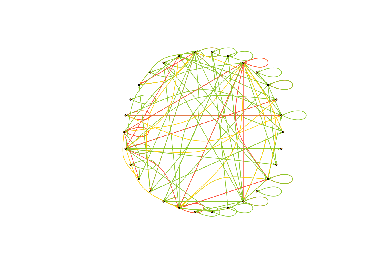
#edge.width=log(E(se.net)$weight+0.1)/4 #can set the width of edgeTo delete edges, using - or delete_edges(graph,edges)
To keep the subgraph with specific edges, using subgraph.edges(graph, eids, delete.vertices = FALSE)
set.seed(1)
#fix the layout
l=layout_in_circle(se.net)
plot(se.net,edge.arrow.size=0.2,layout=l,vertex.shape="none")
#delete the edges
se.net.to=se.net-E(se.net)[E(se.net)$Reciptype%in%c("cc","bcc")]
#se.net.to=delete.edges(se.net,E(se.net)[E(se.net)$Reciptype%in%c("cc","bcc")]) #another way to delete
#se.net.to=subgraph.edges(se.net,E(se.net)[E(se.net)$Reciptype=="to"],delete.vertices = FALSE) # keep the subgraph
se.net.cc=se.net-E(se.net)[E(se.net)$Reciptype%in%c("to","bcc")]
se.net.bcc=se.net-E(se.net)[E(se.net)$Reciptype%in%c("to","cc")]
par(mfrow=c(1,3))
plot(se.net.to,edge.arrow.size=0.2,layout=l,vertex.shape="none")
plot(se.net.cc,edge.arrow.size=0.2,layout=l,vertex.shape="none")
plot(se.net.bcc,edge.arrow.size=0.2,layout=l,vertex.shape="none")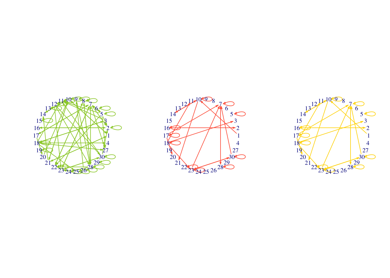
5.5 ggplot2 version for network visualization
5.5.1 ggnet2,geomnet,ggnetwork
ggplot2 version for network visualization
ggnet2: https://briatte.github.io/ggnet/geomnet: https://github.com/sctyner/geomnet https://cran.r-project.org/web/packages/geomnet/geomnet.pdfggnetwork: https://briatte.github.io/ggnetwork/
Comparison among the three R packages: https://journal.r-project.org/archive/2017/RJ-2017-023/RJ-2017-023.pdf
All based on ggplot2 and network
ggnet2has similar syntax asplot. easy to use.geomnetadd available layergeom_netinggplot2. use dataframe as input. can interact withplotlyggnetwork(preferred) is most flexible. advantages on dynamic network.
5.5.2 football data
#install.packages("GGally")
library("GGally")
#install.packages("geomnet")
library("geomnet")
#install.packages("ggnetwork")
library("ggnetwork")
library("statnet")
# load the data
data("football",package = "geomnet")
rownames(football$vertices) <-football$vertices$label
# create network from edge list
fb.net=network::network(football$edges[,1:2])
# add vertex attribute: the conference the team is in
fb.net %v% "conf" <-football$vertices[network.vertex.names(fb.net), "value"]
# add edge attribute: whether two teams belong to the same conference
set.edge.attribute(fb.net, "same.conf",football$edges$same.conf)
set.edge.attribute(fb.net, "lty", ifelse(fb.net %e% "same.conf" == 1, 1, 2))5.5.3 ggnet2
Features:
- Input:
networkobject - Available detailed tutorial. https://briatte.github.io/ggnet/
- Syntax is similar to
plot - Output the underlying organized struture (positions of nodes). Easy to add
geom_xx
Issues:
- No curved edges
- No self-loops
- No complex graphs
- For evolving graphs, cannot provide multiple facet directly. Need to fix the placement coordinates.
set.seed(3212019)
pggnet2=ggnet2(fb.net, # input `network` object
       mode = "fruchtermanreingold", # layout from `network` pkg
       layout.par = list(cell.jitter=0.75), #can pass the layout args
       #node attribute
       node.color = "conf",
       palette = "Paired", #palette="Set3",
       node.size=5,
       #node.size="degree",
       #size.cut=3, # cut the size to three categories using quantiles
       #size="conf",
       #to manual mapping the size: size.palette=c("Atlantic Coast"=1,...),
       #node.shape = "conf",
       node.alpha = 0.5,
       #node.label = TRUE,
       #edge
       edge.color = c("color", "grey50"), #1st value: same col as node for same group. else 2nd args.
       edge.alpha = 0.5,
       edge.size=0.3,
       edge.lty = "lty",
       #edge.label = 1,
       #edge.label.size=1,
       #legend
       color.legend = "Conference",
       #legend.size = 10,
       #legend.position = "bottom")
)+
  geom_point(aes(color = color), size = 3) # can be treat as ggplot object and add geom_xx layer
pggnet2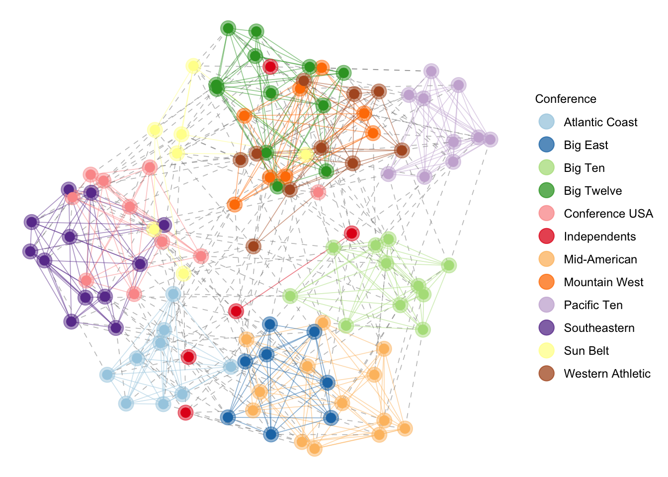
## treat it as dataframe to add geom_xx layer
pggnet2$data%>%names()
## [1] "label" "alpha" "color" "shape" "size" "x" "y"5.5.4 geomnet
Features:
- Input: dataframe
- Allow self-loops
- Allow facet (cannot fix the nodes)
Issues:
- No available detailed tutorial.
- The underlying structured is not available. It is wrapped as a whole. (eg. if setting alpha, is for both nodes and edges; do not provide the positions of points)
- Obey the
ggplot2syntax “strictly”, less flexible
#merge the vertex and edges
ver.conf=football$vertices%>%mutate(from=label)%>%select(-label)
fb.df=left_join(football$edges,ver.conf,by="from")
# create data plot
set.seed(3212019)
pgeomnet=
  ggplot(data = fb.df, # input: dataframe
  aes(from_id = from, to_id = to)) +
  geom_net(layout.alg = 'fruchtermanreingold',
  aes(colour = value, group = value,
  linetype = factor(same.conf != 1)),
  linewidth = 0.5,
  size = 5, vjust = -0.75, alpha = 1) +
  theme_net() +
  #theme(legend.position = "bottom") +
  scale_colour_brewer("Conference", palette = "Paired") +
  guides(linetype = FALSE)
pgeomnet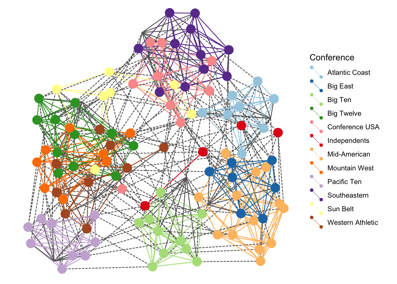
## the underlying dataframe is not point + line
pgeomnet$data%>%names()
## [1] "from" "to" "same.conf" "value"5.5.5 ggnetwork
Features:
- Available detailed tutorial, https://briatte.github.io/ggnetwork/
- Input:
igraph(needlibrary(intergraph)) ornetworkobject - Syntax is super userfriendly.
ggnetworkprovide the underlying dataframe- use
geom_edgesandgeom_nodesseparately; can set edge/node-specific mapping within thegeom_xx - for labels
geom_(node/edge)(text/label)[_repel]:geom_nodetext,geom_nodelabel,geom_nodetext_repel,geom_nodelabel_repel,geom_edgetext,geom_edgelabel,geom_edgetext_repel,geom_edgelabel_repel
- Allow curve edges (but is compatible with
plotly) - Can represent dynamic networks using
facetwith fixing the positions of node
Issues:
- No self-loops
## igraph object
fb.igra=graph_from_data_frame(football$edges[,1:2],directed = FALSE)
V(fb.igra)$conf=football$vertices[V(fb.igra)$name, "value"]
E(fb.igra)$same.conf=football$edges$same.conf
E(fb.igra)$lty=ifelse(E(fb.igra)$same.conf == 1, 1, 2)
#need to load this for igraph object
#install.packages("intergraph")
library("intergraph")#Tips: ctrl+shift+A to reformat
set.seed(3212019)
pggnetwork=
ggplot(
ggnetwork(# provide the underlying dataframe
fb.igra, #input: network object
layout = "fruchtermanreingold", #layout
cell.jitter = 0.75),
#can pass layout parameter
aes(x, y, xend = xend, yend = yend)
) + #mapping for edges
geom_edges(aes(linetype = as.factor(same.conf)),
#arrow = arrow(length = unit(6, "pt"), type = "closed") #if directed
color = "grey50",
curvature = 0.2,
alpha=0.5
) +
geom_nodes(aes(color = conf),
size = 5,
alpha=0.5) +
scale_color_brewer("Conference",
palette = "Paired") +
scale_linetype_manual(values = c(2, 1)) +
guides(linetype = FALSE) +
theme_blank()+
geom_nodes(aes(color = conf),
size = 3) # can be treat as ggplot object and add geom_xx layer
pggnetwork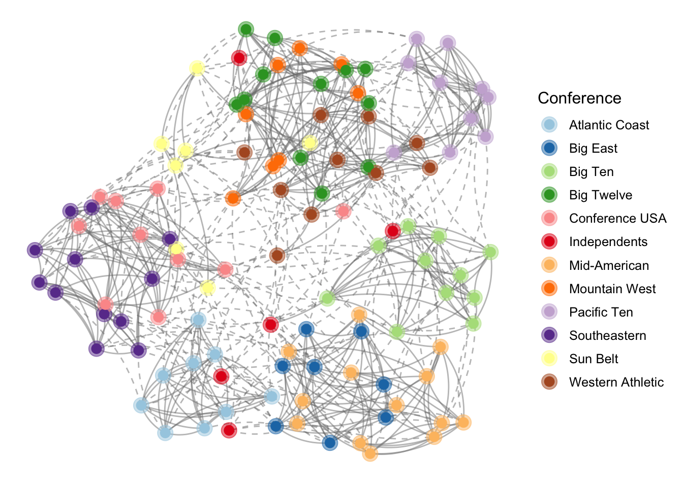
## treat it as dataframe to add geom_xx layer
pggnetwork$data%>%names()
## [1] "x" "y" "conf" "na.x"
## [5] "vertex.names" "xend" "yend" "lty"
## [9] "na.y" "same.conf"5.5.6 Extensions of ggnet2,geomnet,ggnetwork
Since the output is ggplot2 object,
- Interactive network visualization:
ggplot2+plotly - Dynamic network: facet
ggnetwork
5.5.6.1 ggplot2 + plotly
library("plotly")
ggplotly(pggnet2+coord_fixed())%>%hide_guides()ggplotly(pgeomnet+coord_fixed())%>%hide_guides()#if set the `curvature` of the edge, the plotly will not show.
#ggplotly(pggnetwork+coord_fixed())%>%hide_guides()
pggnetwork2=
ggplot(
ggnetwork(# provide the underlying dataframe
fb.igra, #input: network object
layout = "fruchtermanreingold", #layout
cell.jitter = 0.75),
#can pass layout parameter
aes(x, y, xend = xend, yend = yend)
) + #mapping for edges
geom_edges(aes(linetype = as.factor(same.conf)),
#arrow = arrow(length = unit(6, "pt"), type = "closed") #if directed
color = "grey50",
#curvature = 0.2,
alpha=0.5
) +
geom_nodes(aes(color = conf),
size = 5,
alpha=0.5) +
scale_color_brewer("Conference",
palette = "Paired") +
scale_linetype_manual(values = c(2, 1)) +
guides(linetype = FALSE) +
theme_blank()+
geom_nodes(aes(color = conf),
size = 3)
ggplotly(pggnetwork2+coord_fixed())%>%hide_guides()5.5.6.2 Facet dynamic network
Recommend using ggnetwork
## create network
names(email$edges)
## [1] "From" "eID" "Date" "Subject" "to"
## [6] "month" "day" "year" "nrecipients"names(email$nodes)## [1] "label" "LastName"
## [3] "FirstName" "BirthDate"
## [5] "BirthCountry" "Gender"
## [7] "CitizenshipCountry" "CitizenshipBasis"
## [9] "CitizenshipStartDate" "PassportCountry"
## [11] "PassportIssueDate" "PassportExpirationDate"
## [13] "CurrentEmploymentType" "CurrentEmploymentTitle"
## [15] "CurrentEmploymentStartDate" "MilitaryServiceBranch"
## [17] "MilitaryDischargeType" "MilitaryDischargeDate"#edgelist: remove emails sent to all employees
edges=email$edges%>%filter(nrecipients < 54)%>%select(From,to,day)
# Create network
em.net <- network(edges[, 1:2])
# assign edge attributes (day)
set.edge.attribute(em.net, "day", edges[, 3])
# assign vertex attributes (employee type)
em.cet <- as.character(email$nodes$CurrentEmploymentType)
names(em.cet) = email$nodes$label
em.net %v% "curr_empl_type" <- em.cet[ network.vertex.names(em.net) ]set.seed(3212019)
ggplot(
ggnetwork(
em.net,
arrow.gap = 0.02,
by = "day",
layout = "kamadakawai"
),
aes(x, y, xend = xend, yend = yend)
) +
geom_edges(
aes(color = curr_empl_type),
alpha = 0.25,
arrow = arrow(length = unit(5, "pt"), type = "closed")
) +
geom_nodes(aes(color = curr_empl_type), size = 1.5) +
scale_color_brewer("Employment Type", palette = "Set1") +
facet_wrap( .~ day, nrow = 2, labeller = "label_both") +
theme_facet(legend.position = "bottom")## Warning in fortify.network(x, ...): duplicated edges detected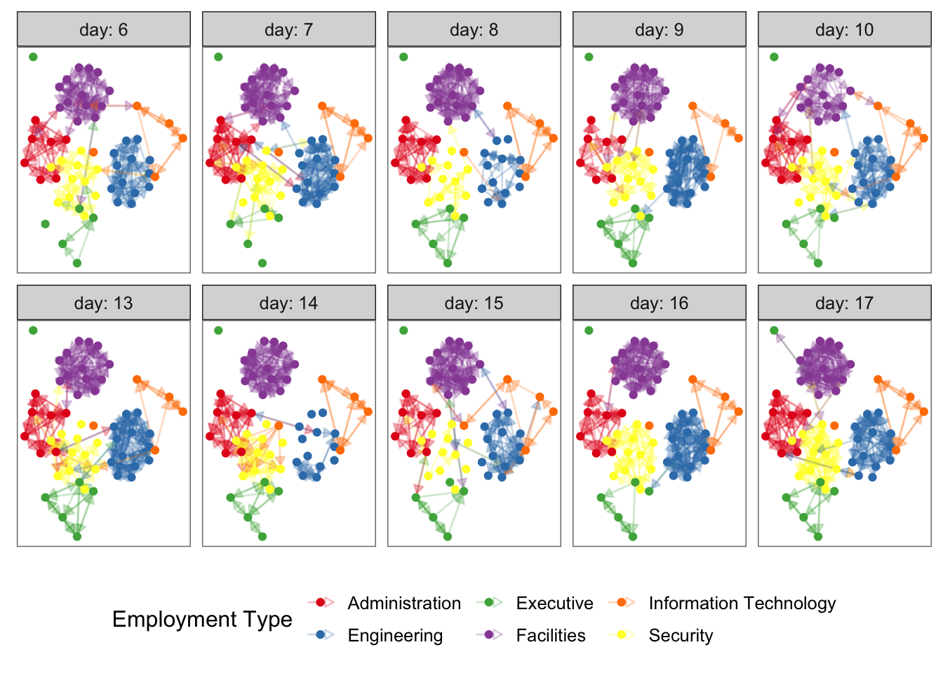
5.6 Interactive network visualization
Apart from the ggplot2 + plotly shown in Chapter @ref{ggplotly}, other available packages:
ggigraphnetworkD3threejsvisNetwork(nice tutorial; Recommended)
5.7 Dynamic network
5.7.1 Introduction
ndtv- Official website: https://cran.r-project.org/web/packages/ndtv/vignettes/ndtv.pdf
- Nice tutorial:
gganimatehttps://gganimate.com/ (ggplot2+gganimate)
5.5.6.3 Comments
The main part of network visualization is the layout of the nodes.All the mentioned R pkg automatically generate the positions of points in the layer. If you want to build a network with pre-specified locations for each node, just draw the points and lines using
plotorggplot.See Chapter 8 Overlaying networks on geographic in http://kateto.net/network-visualization
Figure 5.1: network visualization from kateto