Chapter 3 ERGM (statnet Package)

3.1 Introduction

3.1.1 Outline

Here we only focus on the R package statnet to fit ERGM.

• summary network statistics
• ergm model fitting and interpretation:
• simulate network simulations based on specified model.
• gof, mcmc.diagnostics: Goodness of fit and MCMC diagnostics

3.1.2 statnet

The analytic framework is based on Exponential family Random Graph Models (ergm).

statnet provides a comprehensive framework for ergm-based network modeling, including tools for:

• model estimation
• model-based network simulation
• network visualization
• model evaluation

Powered by Markov chain Monte Carlo (MCMC) algorithm.

3.1.3 References

• Official website (handbook): http://statnet.org/
• Tutorial: https://statnet.org/trac/raw-attachment/wiki/Sunbelt2016/ergm_tutorial.html
• Explore the official websites to find more info

3.2 Preparation

#install.packages("statnet")
library(statnet)

##                Installed  ReposVer Built  
## network        "1.13.0.1" "1.15"   "3.5.0"
## networkDynamic "0.9.0"    "0.10.0" "3.5.0"

library(dplyr)

3.3 summary the network statistics

3.3.1 Dataset

florentine: Florentine Family Marriage and Business Ties Data

data(package="ergm") #see all available dataset in the package
data(florentine) # load flomarriage and flobusiness data
flomarriage # see the details of the network

##  Network attributes:
##   vertices = 16 
##   directed = FALSE 
##   hyper = FALSE 
##   loops = FALSE 
##   multiple = FALSE 
##   bipartite = FALSE 
##   total edges= 20 
##     missing edges= 0 
##     non-missing edges= 20 
## 
##  Vertex attribute names: 
##     priorates totalties vertex.names wealth 
## 
## No edge attributes

class(flomarriage)

## [1] "network"

summary(flomarriage)

## Network attributes:
##   vertices = 16
##   directed = FALSE
##   hyper = FALSE
##   loops = FALSE
##   multiple = FALSE
##   bipartite = FALSE
##  total edges = 20 
##    missing edges = 0 
##    non-missing edges = 20 
##  density = 0.1666667 
## 
## Vertex attributes:
## 
##  priorates:
##    numeric valued attribute
##    attribute summary:
##    Min. 1st Qu.  Median    Mean 3rd Qu.    Max. 
##    0.00    0.00   21.50   25.94   44.75   74.00 
## 
##  totalties:
##    numeric valued attribute
##    attribute summary:
##    Min. 1st Qu.  Median    Mean 3rd Qu.    Max. 
##    1.00    4.75    9.00   13.88   15.00   54.00 
##   vertex.names:
##    character valued attribute
##    16 valid vertex names
## 
##  wealth:
##    numeric valued attribute
##    attribute summary:
##    Min. 1st Qu.  Median    Mean 3rd Qu.    Max. 
##    3.00   17.50   39.00   42.56   48.25  146.00 
## 
## No edge attributes
## 
## Network edgelist matrix:
##       [,1] [,2]
##  [1,]    1    9
##  [2,]    2    6
##  [3,]    2    7
##  [4,]    2    9
##  [5,]    3    5
##  [6,]    3    9
##  [7,]    4    7
##  [8,]    4   11
##  [9,]    4   15
## [10,]    5   11
## [11,]    5   15
## [12,]    7    8
## [13,]    7   16
## [14,]    9   13
## [15,]    9   14
## [16,]    9   16
## [17,]   10   14
## [18,]   11   15
## [19,]   13   15
## [20,]   13   16

set.seed(1)
plot(flomarriage)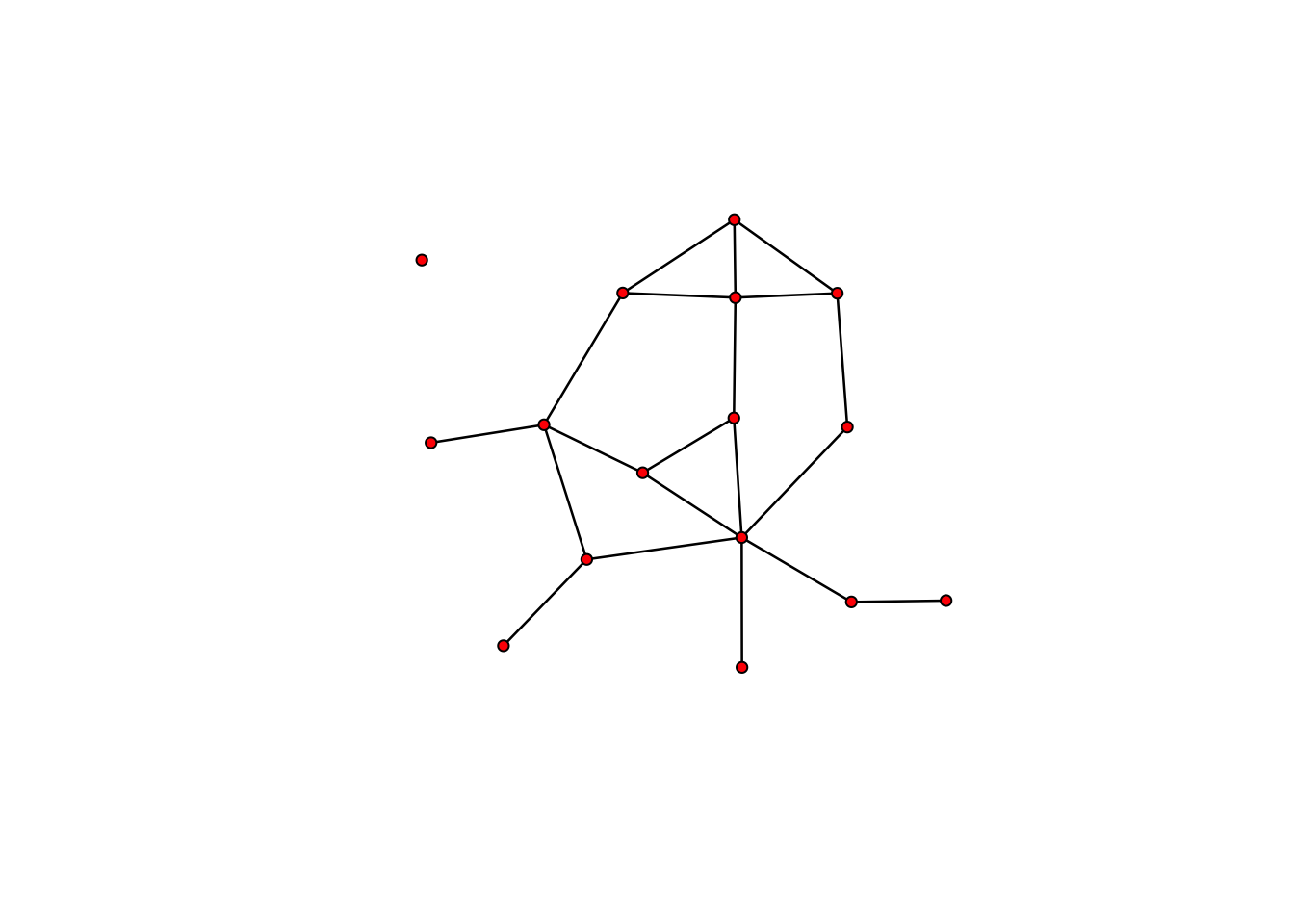

3.3.2 summary

summary(network-object~ergm-terms): provide the statistics of network

summary(flomarriage~edges+triangle+kstar(1:3)+degree(0:5))

##    edges triangle   kstar1   kstar2   kstar3  degree0  degree1  degree2 
##       20        3       40       47       34        1        4        2 
##  degree3  degree4  degree5 
##        6        2        0

3.3.3 directed networks

data(samplk)
samplk3

##  Network attributes:
##   vertices = 18 
##   directed = TRUE 
##   hyper = FALSE 
##   loops = FALSE 
##   multiple = FALSE 
##   bipartite = FALSE 
##   total edges= 56 
##     missing edges= 0 
##     non-missing edges= 56 
## 
##  Vertex attribute names: 
##     cloisterville group vertex.names 
## 
## No edge attributes

set.seed(1)
plot(samplk3)

---

idegree and odegree.

summary(samplk3~idegree(1:3)+odegree(c(2,4))) #indegree and outdegree

## idegree1 idegree2 idegree3 odegree2 odegree4 
##        1        7        2        0        2

3.4 ergm fit ergm model

3.4.1 ERGM

The general form: \(P(g=G)=\frac{exp(\theta'T(G))}{c(\theta)}\)

log-odds of a single edge between node \(i\) and \(j\): \(logit(Y)=\theta'T(G)\)

Similar as regression:

glm(y~x) – ergm(graph~terms) where terms are \(T(\cdot)\)

3.4.2 ergm function.

• Input: formula [netowrk object (adjacency matrix)] ~ [ergm-terms]

#Input
?ergm
class(flomarriage)

## [1] "network"

ergm(flomarriage~edges)%>%summary()

## Starting maximum pseudolikelihood estimation (MPLE):

## Evaluating the predictor and response matrix.

## Maximizing the pseudolikelihood.

## Finished MPLE.

## Stopping at the initial estimate.

## Evaluating log-likelihood at the estimate.

## 
## ==========================
## Summary of model fit
## ==========================
## 
## Formula:   flomarriage ~ edges
## 
## Iterations:  5 out of 20 
## 
## Monte Carlo MLE Results:
##       Estimate Std. Error MCMC % z value Pr(>|z|)    
## edges  -1.6094     0.2449      0  -6.571   <1e-04 ***
## ---
## Signif. codes:  0 '***' 0.001 '**' 0.01 '*' 0.05 '.' 0.1 ' ' 1
## 
##      Null Deviance: 166.4  on 120  degrees of freedom
##  Residual Deviance: 108.1  on 119  degrees of freedom
##  
## AIC: 110.1    BIC: 112.9    (Smaller is better.)

mat=as.sociomatrix(flomarriage)
ergm(mat~edges)%>%summary()

## Starting maximum pseudolikelihood estimation (MPLE):
## Evaluating the predictor and response matrix.
## Maximizing the pseudolikelihood.
## Finished MPLE.
## Stopping at the initial estimate.
## Evaluating log-likelihood at the estimate.

## 
## ==========================
## Summary of model fit
## ==========================
## 
## Formula:   mat ~ edges
## 
## Iterations:  5 out of 20 
## 
## Monte Carlo MLE Results:
##       Estimate Std. Error MCMC % z value Pr(>|z|)    
## edges  -1.6094     0.1732      0  -9.292   <1e-04 ***
## ---
## Signif. codes:  0 '***' 0.001 '**' 0.01 '*' 0.05 '.' 0.1 ' ' 1
## 
##      Null Deviance: 332.7  on 240  degrees of freedom
##  Residual Deviance: 216.3  on 239  degrees of freedom
##  
## AIC: 218.3    BIC: 221.8    (Smaller is better.)

---

• Output: ergm object

• Method on ergm object:

  • class
  • names
  • summary
  • coef
  • coefficients
  • vcov

flomodel.01=ergm(flomarriage~edges)

## Starting maximum pseudolikelihood estimation (MPLE):

## Evaluating the predictor and response matrix.

## Maximizing the pseudolikelihood.

## Finished MPLE.

## Stopping at the initial estimate.

## Evaluating log-likelihood at the estimate.

summary(flomodel.01)

## 
## ==========================
## Summary of model fit
## ==========================
## 
## Formula:   flomarriage ~ edges
## 
## Iterations:  5 out of 20 
## 
## Monte Carlo MLE Results:
##       Estimate Std. Error MCMC % z value Pr(>|z|)    
## edges  -1.6094     0.2449      0  -6.571   <1e-04 ***
## ---
## Signif. codes:  0 '***' 0.001 '**' 0.01 '*' 0.05 '.' 0.1 ' ' 1
## 
##      Null Deviance: 166.4  on 120  degrees of freedom
##  Residual Deviance: 108.1  on 119  degrees of freedom
##  
## AIC: 110.1    BIC: 112.9    (Smaller is better.)

class(flomodel.01)

## [1] "ergm"

names(flomodel.01)

##  [1] "coef"         "iterations"   "MCMCtheta"    "gradient"    
##  [5] "hessian"      "covar"        "failure"      "est.cov"     
##  [9] "glm"          "glm.null"     "theta1"       "offset"      
## [13] "drop"         "estimable"    "network"      "reference"   
## [17] "newnetwork"   "formula"      "constrained"  "constraints" 
## [21] "target.stats" "etamap"       "target.esteq" "estimate"    
## [25] "control"      "null.lik"     "mle.lik"

flomodel.01$coef

##     edges 
## -1.609438

coef(flomodel.01)

##     edges 
## -1.609438

coefficients(flomodel.01)

## Warning: You appear to be calling coef.ergm() directly. coef.ergm() is a
## method, and will not be exported in a future version of 'ergm'. Use coef()
## instead, or getS3method() if absolutely necessary.

##     edges 
## -1.609438

vcov(flomodel.01) #variance-covariance matrix of the main parameters

##            edges
## edges 0.05999985

vcov(flomodel.01)%>%sqrt()

##           edges
## edges 0.2449487

vcov(ergm(flomarriage~edges+triangle))

## Starting maximum pseudolikelihood estimation (MPLE):
## Evaluating the predictor and response matrix.
## Maximizing the pseudolikelihood.
## Finished MPLE.
## Starting Monte Carlo maximum likelihood estimation (MCMLE):
## Iteration 1 of at most 20:
## Optimizing with step length 1.
## The log-likelihood improved by 0.002922.
## Step length converged once. Increasing MCMC sample size.
## Iteration 2 of at most 20:
## Optimizing with step length 1.
## The log-likelihood improved by 0.0006953.
## Step length converged twice. Stopping.
## Finished MCMLE.
## Evaluating log-likelihood at the estimate. Using 20 bridges: 1 2 3 4 5 6 7 8 9 10 11 12 13 14 15 16 17 18 19 20 .
## This model was fit using MCMC.  To examine model diagnostics and check for degeneracy, use the mcmc.diagnostics() function.

##               edges   triangle
## edges     0.1242829 -0.1573260
## triangle -0.1573260  0.3539089

3.4.3 ergm-terms

See the full list of ergm-terms

help('ergm-terms')

3.4.3.1 Erdos-Renyi model G(n,p) model: include edges term

Edge included in the graph with prob \(p\): \(Pr(A=a|p)=\prod p^{a_{ij}}(1-p)^{1-a_{ij}}\)

Rewrite Erdos-Renyi model in ERGM form: \(T(G)=\#edges\), \(\theta=log \frac{p}{1-p}\)

3.4.3.2 Interpretation of the parameter

Interpretation (similar when you interpret glm):

• edges: If the number of edges increase 1, the log-odds of any edge existing is -1.6094.

• \(p<\alpha\): parameter does not equal to 0 significantly,

• Null Deviance: The null deviance in the ergm output appears to be based on an Erdos-Renyi random graph with p = 0.5.

• Residual Deviance: 2 times difference of loglik (saturated model - our model) (smaller is better)

• AIC, BIC: -loglik+penalty(#parameter)

flomodel.01=ergm(flomarriage~edges) #similar as regression lm(y~x)

## Starting maximum pseudolikelihood estimation (MPLE):

## Evaluating the predictor and response matrix.

## Maximizing the pseudolikelihood.

## Finished MPLE.

## Stopping at the initial estimate.

## Evaluating log-likelihood at the estimate.

summary(flomodel.01) 

## 
## ==========================
## Summary of model fit
## ==========================
## 
## Formula:   flomarriage ~ edges
## 
## Iterations:  5 out of 20 
## 
## Monte Carlo MLE Results:
##       Estimate Std. Error MCMC % z value Pr(>|z|)    
## edges  -1.6094     0.2449      0  -6.571   <1e-04 ***
## ---
## Signif. codes:  0 '***' 0.001 '**' 0.01 '*' 0.05 '.' 0.1 ' ' 1
## 
##      Null Deviance: 166.4  on 120  degrees of freedom
##  Residual Deviance: 108.1  on 119  degrees of freedom
##  
## AIC: 110.1    BIC: 112.9    (Smaller is better.)

flomodel.01$coef/(1+exp(flomodel.01$coef)) # prob of an edge exists

##     edges 
## -1.341198

-2*(flomodel.01$mle.lik)+2 #AIC: -2loglik+2k

## 'log Lik.' 110.1347 (df=1)

-2*(flomodel.01$mle.lik)+log(16*15/2) #BIC:-2loglik+klog(n)

## 'log Lik.' 112.9222 (df=1)

pchisq(108.1 , df=119, lower.tail=FALSE) # H0: our model fits well. The smaller the better. Accept H0.

## [1] 0.7535728

3.4.3.3 Include triangle terms

Include number of triangles as a measure of clustering.

flomodel.02=ergm(flomarriage~edges+triangle)

## Starting maximum pseudolikelihood estimation (MPLE):

## Evaluating the predictor and response matrix.

## Maximizing the pseudolikelihood.

## Finished MPLE.

## Starting Monte Carlo maximum likelihood estimation (MCMLE):

## Iteration 1 of at most 20:

## Optimizing with step length 1.

## The log-likelihood improved by 0.00888.

## Step length converged once. Increasing MCMC sample size.

## Iteration 2 of at most 20:

## Optimizing with step length 1.

## The log-likelihood improved by 0.000148.

## Step length converged twice. Stopping.

## Finished MCMLE.

## Evaluating log-likelihood at the estimate. Using 20 bridges: 1 2 3 4 5 6 7 8 9 10 11 12 13 14 15 16 17 18 19 20 .
## This model was fit using MCMC.  To examine model diagnostics and check for degeneracy, use the mcmc.diagnostics() function.

summary(flomodel.02)

## 
## ==========================
## Summary of model fit
## ==========================
## 
## Formula:   flomarriage ~ edges + triangle
## 
## Iterations:  2 out of 20 
## 
## Monte Carlo MLE Results:
##          Estimate Std. Error MCMC % z value Pr(>|z|)    
## edges     -1.6737     0.3578      0  -4.677   <1e-04 ***
## triangle   0.1490     0.6029      0   0.247    0.805    
## ---
## Signif. codes:  0 '***' 0.001 '**' 0.01 '*' 0.05 '.' 0.1 ' ' 1
## 
##      Null Deviance: 166.4  on 120  degrees of freedom
##  Residual Deviance: 108.1  on 118  degrees of freedom
##  
## AIC: 112.1    BIC: 117.6    (Smaller is better.)

• Coefficients: -1.6744\(\times\)#of edges+0.1497\(\times\)#of triangles

• triangle is not significant

• AIC, BIC: larger than that of ER model

3.4.3.4 Include nodal covariates: nodecov

Using nodecov to include continuous nodal covariates

flomarriage

##  Network attributes:
##   vertices = 16 
##   directed = FALSE 
##   hyper = FALSE 
##   loops = FALSE 
##   multiple = FALSE 
##   bipartite = FALSE 
##   total edges= 20 
##     missing edges= 0 
##     non-missing edges= 20 
## 
##  Vertex attribute names: 
##     priorates totalties vertex.names wealth 
## 
## No edge attributes

wealth=flomarriage %v% 'wealth' # %v% get the vertex attributes
set.seed(1)
plot(flomarriage, vertex.cex=wealth/25, main="Florentine marriage by wealth", cex.main=0.8)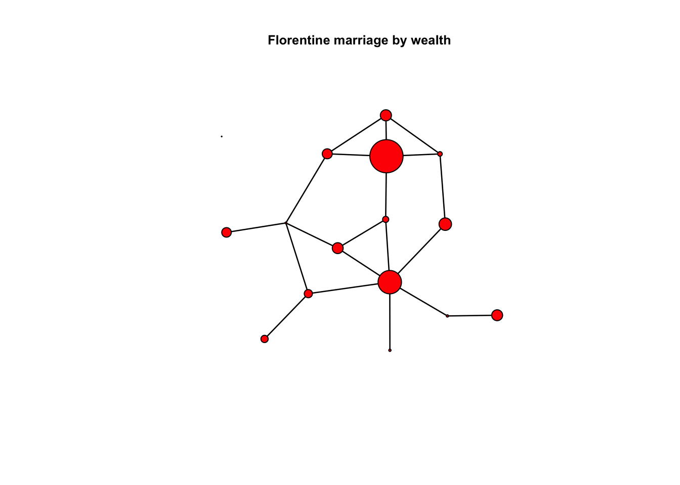

flomodel.03=ergm(flomarriage~edges+nodecov('wealth'))

## Starting maximum pseudolikelihood estimation (MPLE):

## Evaluating the predictor and response matrix.

## Maximizing the pseudolikelihood.

## Finished MPLE.

## Stopping at the initial estimate.

## Evaluating log-likelihood at the estimate.

summary(flomodel.03)

## 
## ==========================
## Summary of model fit
## ==========================
## 
## Formula:   flomarriage ~ edges + nodecov("wealth")
## 
## Iterations:  4 out of 20 
## 
## Monte Carlo MLE Results:
##                 Estimate Std. Error MCMC % z value Pr(>|z|)    
## edges          -2.594929   0.536056      0  -4.841   <1e-04 ***
## nodecov.wealth  0.010546   0.004674      0   2.256   0.0241 *  
## ---
## Signif. codes:  0 '***' 0.001 '**' 0.01 '*' 0.05 '.' 0.1 ' ' 1
## 
##      Null Deviance: 166.4  on 120  degrees of freedom
##  Residual Deviance: 103.1  on 118  degrees of freedom
##  
## AIC: 107.1    BIC: 112.7    (Smaller is better.)

Interpretation: -2.594929 # of edges + 0.010546 wealth of node i + 0.010546 wealth of node j

3.4.3.5 Include transformation of continuous nodal covariates

flomodel.04=ergm(flomarriage~edges+absdiff("wealth"))

## Starting maximum pseudolikelihood estimation (MPLE):

## Evaluating the predictor and response matrix.

## Maximizing the pseudolikelihood.

## Finished MPLE.

## Stopping at the initial estimate.

## Evaluating log-likelihood at the estimate.

summary(flomodel.04)

## 
## ==========================
## Summary of model fit
## ==========================
## 
## Formula:   flomarriage ~ edges + absdiff("wealth")
## 
## Iterations:  4 out of 20 
## 
## Monte Carlo MLE Results:
##                 Estimate Std. Error MCMC % z value Pr(>|z|)    
## edges          -2.302042   0.401906      0  -5.728   <1e-04 ***
## absdiff.wealth  0.015519   0.006157      0   2.521   0.0117 *  
## ---
## Signif. codes:  0 '***' 0.001 '**' 0.01 '*' 0.05 '.' 0.1 ' ' 1
## 
##      Null Deviance: 166.4  on 120  degrees of freedom
##  Residual Deviance: 102.0  on 118  degrees of freedom
##  
## AIC: 106    BIC: 111.5    (Smaller is better.)

3.4.3.6 Include transformation of continuous nodal covariates

flomodel.05=ergm(flomarriage~edges+nodecov('wealth')+nodecov('wealth',transform=function(x) x^2))

## Starting maximum pseudolikelihood estimation (MPLE):

## Evaluating the predictor and response matrix.

## Maximizing the pseudolikelihood.

## Finished MPLE.

## Stopping at the initial estimate.

## Evaluating log-likelihood at the estimate.

summary(flomodel.05)

## 
## ==========================
## Summary of model fit
## ==========================
## 
## Formula:   flomarriage ~ edges + nodecov("wealth") + nodecov("wealth", transform = function(x) x^2)
## 
## Iterations:  4 out of 20 
## 
## Monte Carlo MLE Results:
##                    Estimate Std. Error MCMC % z value Pr(>|z|)   
## edges            -2.904e+00  9.313e-01      0  -3.119  0.00182 **
## nodecov.wealth    1.730e-02  1.695e-02      0   1.021  0.30737   
## nodecov.wealth.1 -4.459e-05  1.073e-04      0  -0.416  0.67768   
## ---
## Signif. codes:  0 '***' 0.001 '**' 0.01 '*' 0.05 '.' 0.1 ' ' 1
## 
##      Null Deviance: 166.4  on 120  degrees of freedom
##  Residual Deviance: 102.9  on 117  degrees of freedom
##  
## AIC: 108.9    BIC: 117.3    (Smaller is better.)

3.4.3.7 Include other possible ergm-terms

flomodel.06=ergm(flomarriage~kstar(1:2) + absdiff("wealth"))

## Starting maximum pseudolikelihood estimation (MPLE):

## Evaluating the predictor and response matrix.

## Maximizing the pseudolikelihood.

## Finished MPLE.

## Starting Monte Carlo maximum likelihood estimation (MCMLE):

## Iteration 1 of at most 20:

## Optimizing with step length 1.

## The log-likelihood improved by 0.01795.

## Step length converged once. Increasing MCMC sample size.

## Iteration 2 of at most 20:

## Optimizing with step length 1.

## The log-likelihood improved by 0.001918.

## Step length converged twice. Stopping.

## Finished MCMLE.

## Evaluating log-likelihood at the estimate. Using 20 bridges: 1 2 3 4 5 6 7 8 9 10 11 12 13 14 15 16 17 18 19 20 .
## This model was fit using MCMC.  To examine model diagnostics and check for degeneracy, use the mcmc.diagnostics() function.

summary(flomodel.06)

## 
## ==========================
## Summary of model fit
## ==========================
## 
## Formula:   flomarriage ~ kstar(1:2) + absdiff("wealth")
## 
## Iterations:  2 out of 20 
## 
## Monte Carlo MLE Results:
##                 Estimate Std. Error MCMC % z value Pr(>|z|)  
## kstar1         -0.857799   0.455348      0  -1.884   0.0596 .
## kstar2         -0.162150   0.224192      0  -0.723   0.4695  
## absdiff.wealth  0.019244   0.008719      0   2.207   0.0273 *
## ---
## Signif. codes:  0 '***' 0.001 '**' 0.01 '*' 0.05 '.' 0.1 ' ' 1
## 
##      Null Deviance: 166.4  on 120  degrees of freedom
##  Residual Deviance: 101.3  on 117  degrees of freedom
##  
## AIC: 107.3    BIC: 115.7    (Smaller is better.)

summary(ergm(flomarriage~kstar(c(1,3)) + absdiff("wealth")))

## Starting maximum pseudolikelihood estimation (MPLE):
## Evaluating the predictor and response matrix.
## Maximizing the pseudolikelihood.
## Finished MPLE.
## Starting Monte Carlo maximum likelihood estimation (MCMLE):
## Iteration 1 of at most 20:
## Optimizing with step length 1.
## The log-likelihood improved by 0.01691.
## Step length converged once. Increasing MCMC sample size.
## Iteration 2 of at most 20:
## Optimizing with step length 1.
## The log-likelihood improved by 0.001825.
## Step length converged twice. Stopping.
## Finished MCMLE.
## Evaluating log-likelihood at the estimate. Using 20 bridges: 1 2 3 4 5 6 7 8 9 10 11 12 13 14 15 16 17 18 19 20 .
## This model was fit using MCMC.  To examine model diagnostics and check for degeneracy, use the mcmc.diagnostics() function.

## 
## ==========================
## Summary of model fit
## ==========================
## 
## Formula:   flomarriage ~ kstar(c(1, 3)) + absdiff("wealth")
## 
## Iterations:  2 out of 20 
## 
## Monte Carlo MLE Results:
##                 Estimate Std. Error MCMC % z value Pr(>|z|)    
## kstar1         -1.054277   0.261968      0  -4.024   <1e-04 ***
## kstar3         -0.086239   0.111865      0  -0.771   0.4408    
## absdiff.wealth  0.020937   0.009522      0   2.199   0.0279 *  
## ---
## Signif. codes:  0 '***' 0.001 '**' 0.01 '*' 0.05 '.' 0.1 ' ' 1
## 
##      Null Deviance: 166.4  on 120  degrees of freedom
##  Residual Deviance: 101.0  on 117  degrees of freedom
##  
## AIC: 107    BIC: 115.4    (Smaller is better.)

3.4.3.8 Include categorical nodal covariates: nodefactor

data("faux.mesa.high")
mesa=faux.mesa.high
mesa # grade, race, sex are discrete vertex attribute

##  Network attributes:
##   vertices = 205 
##   directed = FALSE 
##   hyper = FALSE 
##   loops = FALSE 
##   multiple = FALSE 
##   bipartite = FALSE 
##   total edges= 203 
##     missing edges= 0 
##     non-missing edges= 203 
## 
##  Vertex attribute names: 
##     Grade Race Sex 
## 
## No edge attributes

plot(mesa, vertex.col='Grade')
legend('bottomleft',fill=7:12,legend=paste('Grade',7:12),cex=0.75)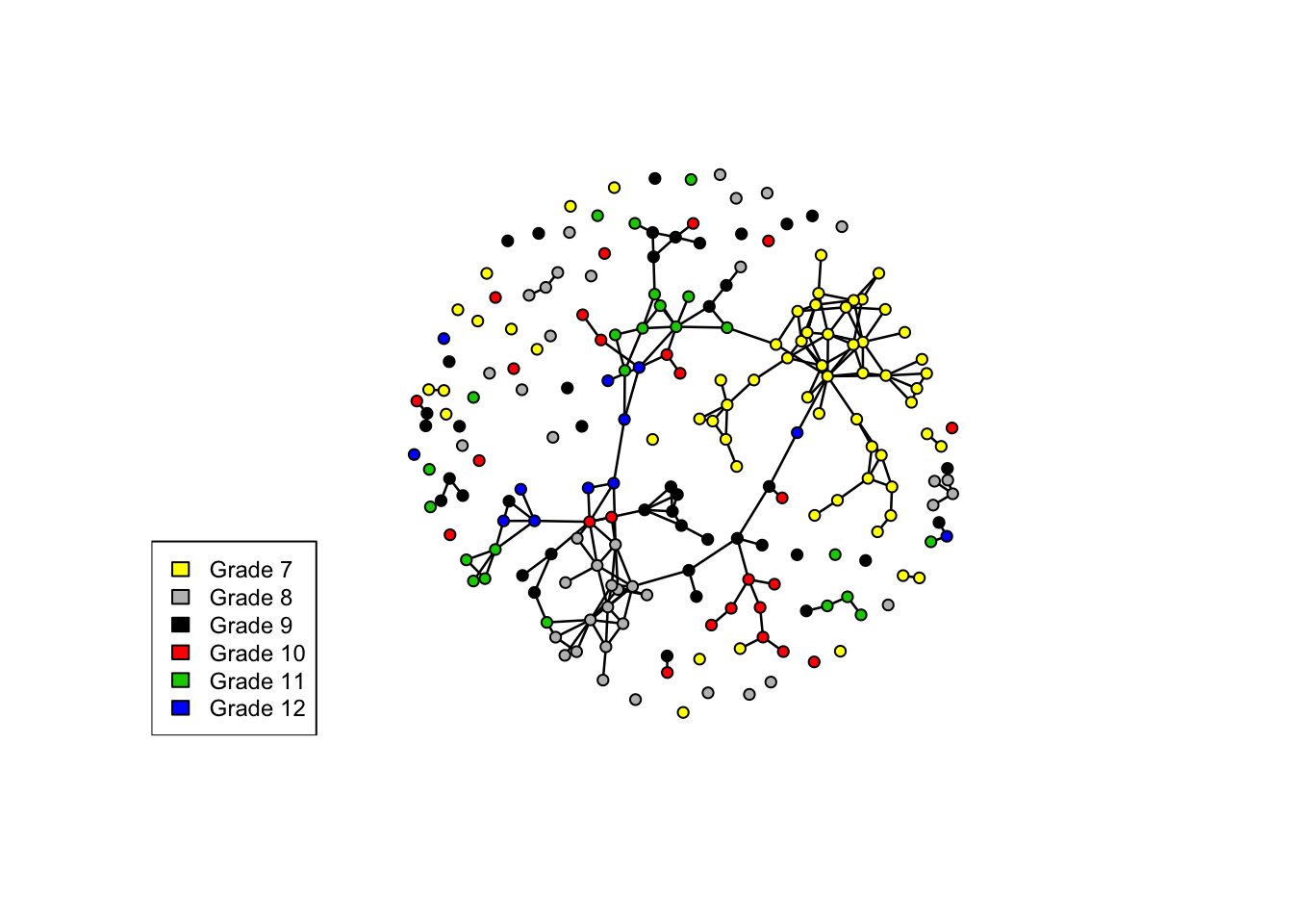

3.4.3.9 Include discrete nodal covariates: nodefactor

fauxmodel.01=ergm(mesa ~edges + nodecov('Grade'))

## Starting maximum pseudolikelihood estimation (MPLE):

## Evaluating the predictor and response matrix.

## Maximizing the pseudolikelihood.

## Finished MPLE.

## Stopping at the initial estimate.

## Evaluating log-likelihood at the estimate.

summary(fauxmodel.01)

## 
## ==========================
## Summary of model fit
## ==========================
## 
## Formula:   mesa ~ edges + nodecov("Grade")
## 
## Iterations:  7 out of 20 
## 
## Monte Carlo MLE Results:
##               Estimate Std. Error MCMC % z value Pr(>|z|)    
## edges         -3.64578    0.56757      0  -6.424   <1e-04 ***
## nodecov.Grade -0.05650    0.03274      0  -1.726   0.0844 .  
## ---
## Signif. codes:  0 '***' 0.001 '**' 0.01 '*' 0.05 '.' 0.1 ' ' 1
## 
##      Null Deviance: 28987  on 20910  degrees of freedom
##  Residual Deviance:  2283  on 20908  degrees of freedom
##  
## AIC: 2287    BIC: 2303    (Smaller is better.)

fauxmodel.02=ergm(mesa ~edges + nodefactor('Grade'))

## Starting maximum pseudolikelihood estimation (MPLE):
## Evaluating the predictor and response matrix.
## Maximizing the pseudolikelihood.
## Finished MPLE.
## Stopping at the initial estimate.
## Evaluating log-likelihood at the estimate.

summary(fauxmodel.02)

## 
## ==========================
## Summary of model fit
## ==========================
## 
## Formula:   mesa ~ edges + nodefactor("Grade")
## 
## Iterations:  6 out of 20 
## 
## Monte Carlo MLE Results:
##                     Estimate Std. Error MCMC % z value Pr(>|z|)    
## edges               -4.17784    0.14696      0 -28.428  < 1e-04 ***
## nodefactor.Grade.8  -0.27924    0.14209      0  -1.965  0.04938 *  
## nodefactor.Grade.9  -0.47364    0.14912      0  -3.176  0.00149 ** 
## nodefactor.Grade.10 -0.54653    0.18641      0  -2.932  0.00337 ** 
## nodefactor.Grade.11 -0.19281    0.16550      0  -1.165  0.24401    
## nodefactor.Grade.12 -0.05704    0.20739      0  -0.275  0.78330    
## ---
## Signif. codes:  0 '***' 0.001 '**' 0.01 '*' 0.05 '.' 0.1 ' ' 1
## 
##      Null Deviance: 28987  on 20910  degrees of freedom
##  Residual Deviance:  2269  on 20904  degrees of freedom
##  
## AIC: 2281    BIC: 2329    (Smaller is better.)

3.4.3.10 Include other terms: eg. homophily

help('ergm-terms') # check all the possible ergm terms

3.4.3.11 Include other terms: eg. homophily

nodematch: Uniform homophily and differential homophily

uniform homophily(diff=FALSE), adds one network statistic to the model, which counts the number of edges (i,j) for which attrname(i)==attrname(j).

differential homophily(diff=TRUE), p(#of unique values of the attrname attribute) network statistics are added to the model.

The kth such statistic counts the number of edges (i,j) for which attrname(i) == attrname(j) == value(k), where value(k) is the kth smallest unique value of the attrname attribute.

When multiple attribute names are given, the statistic counts only ties for which all of the attributes match.

?nodematch
fauxmodel.03 <- ergm(mesa ~edges + nodematch('Grade',diff=F) )

## Starting maximum pseudolikelihood estimation (MPLE):

## Evaluating the predictor and response matrix.

## Maximizing the pseudolikelihood.

## Finished MPLE.

## Stopping at the initial estimate.

## Evaluating log-likelihood at the estimate.

summary(fauxmodel.03)

## 
## ==========================
## Summary of model fit
## ==========================
## 
## Formula:   mesa ~ edges + nodematch("Grade", diff = F)
## 
## Iterations:  8 out of 20 
## 
## Monte Carlo MLE Results:
##                 Estimate Std. Error MCMC % z value Pr(>|z|)    
## edges            -6.0340     0.1583      0  -38.12   <1e-04 ***
## nodematch.Grade   2.8310     0.1773      0   15.96   <1e-04 ***
## ---
## Signif. codes:  0 '***' 0.001 '**' 0.01 '*' 0.05 '.' 0.1 ' ' 1
## 
##      Null Deviance: 28987  on 20910  degrees of freedom
##  Residual Deviance:  1940  on 20908  degrees of freedom
##  
## AIC: 1944    BIC: 1959    (Smaller is better.)

mixingmatrix(mesa, "Race") # reason for Inf

## Note:  Marginal totals can be misleading
##  for undirected mixing matrices.
##       Black Hisp NatAm Other White
## Black     0    8    13     0     5
## Hisp      8   53    41     1    22
## NatAm    13   41    46     0    10
## Other     0    1     0     0     0
## White     5   22    10     0     4

fauxmodel.04 <- ergm(mesa ~edges + nodematch('Grade',diff=T) )

## Starting maximum pseudolikelihood estimation (MPLE):
## Evaluating the predictor and response matrix.
## Maximizing the pseudolikelihood.
## Finished MPLE.
## Stopping at the initial estimate.
## Evaluating log-likelihood at the estimate.

summary(fauxmodel.04)

## 
## ==========================
## Summary of model fit
## ==========================
## 
## Formula:   mesa ~ edges + nodematch("Grade", diff = T)
## 
## Iterations:  8 out of 20 
## 
## Monte Carlo MLE Results:
##                    Estimate Std. Error MCMC % z value Pr(>|z|)    
## edges               -6.0340     0.1583      0 -38.117   <1e-04 ***
## nodematch.Grade.7    2.8471     0.1973      0  14.427   <1e-04 ***
## nodematch.Grade.8    2.9145     0.2381      0  12.240   <1e-04 ***
## nodematch.Grade.9    2.4385     0.2641      0   9.234   <1e-04 ***
## nodematch.Grade.10   2.5579     0.3736      0   6.846   <1e-04 ***
## nodematch.Grade.11   3.3104     0.2962      0  11.176   <1e-04 ***
## nodematch.Grade.12   3.7315     0.4565      0   8.174   <1e-04 ***
## ---
## Signif. codes:  0 '***' 0.001 '**' 0.01 '*' 0.05 '.' 0.1 ' ' 1
## 
##      Null Deviance: 28987  on 20910  degrees of freedom
##  Residual Deviance:  1928  on 20903  degrees of freedom
##  
## AIC: 1942    BIC: 1998    (Smaller is better.)

fauxmodel.04 <- ergm(mesa ~edges + nodematch('Grade',diff=T,keep=c(2,4)) )

## Starting maximum pseudolikelihood estimation (MPLE):
## Evaluating the predictor and response matrix.
## Maximizing the pseudolikelihood.
## Finished MPLE.
## Stopping at the initial estimate.
## Evaluating log-likelihood at the estimate.

summary(fauxmodel.04)

## 
## ==========================
## Summary of model fit
## ==========================
## 
## Formula:   mesa ~ edges + nodematch("Grade", diff = T, keep = c(2, 4))
## 
## Iterations:  7 out of 20 
## 
## Monte Carlo MLE Results:
##                    Estimate Std. Error MCMC % z value Pr(>|z|)    
## edges              -4.80539    0.07913      0 -60.727  < 1e-04 ***
## nodematch.Grade.8   1.68584    0.19469      0   8.659  < 1e-04 ***
## nodematch.Grade.10  1.32930    0.34758      0   3.824 0.000131 ***
## ---
## Signif. codes:  0 '***' 0.001 '**' 0.01 '*' 0.05 '.' 0.1 ' ' 1
## 
##      Null Deviance: 28987  on 20910  degrees of freedom
##  Residual Deviance:  2225  on 20907  degrees of freedom
##  
## AIC: 2231    BIC: 2255    (Smaller is better.)

fauxmodel.05 <- ergm(mesa ~edges + nodematch('Grade',diff=T)+ nodematch('Race',diff=T) )

## Observed statistic(s) nodematch.Race.Black and nodematch.Race.Other are at their smallest attainable values. Their coefficients will be fixed at -Inf.
## Starting maximum pseudolikelihood estimation (MPLE):
## Evaluating the predictor and response matrix.
## Maximizing the pseudolikelihood.
## Finished MPLE.
## Stopping at the initial estimate.
## Evaluating log-likelihood at the estimate.

summary(fauxmodel.05)

## 
## ==========================
## Summary of model fit
## ==========================
## 
## Formula:   mesa ~ edges + nodematch("Grade", diff = T) + nodematch("Race", 
##     diff = T)
## 
## Iterations:  8 out of 20 
## 
## Monte Carlo MLE Results:
##                      Estimate Std. Error MCMC % z value Pr(>|z|)    
## edges                 -6.2328     0.1742      0 -35.785   <1e-04 ***
## nodematch.Grade.7      2.8740     0.1981      0  14.509   <1e-04 ***
## nodematch.Grade.8      2.8788     0.2391      0  12.038   <1e-04 ***
## nodematch.Grade.9      2.4642     0.2647      0   9.310   <1e-04 ***
## nodematch.Grade.10     2.5692     0.3770      0   6.815   <1e-04 ***
## nodematch.Grade.11     3.2921     0.2978      0  11.057   <1e-04 ***
## nodematch.Grade.12     3.8376     0.4592      0   8.357   <1e-04 ***
## nodematch.Race.Black     -Inf     0.0000      0    -Inf   <1e-04 ***
## nodematch.Race.Hisp    0.0679     0.1737      0   0.391   0.6959    
## nodematch.Race.NatAm   0.9817     0.1842      0   5.329   <1e-04 ***
## nodematch.Race.Other     -Inf     0.0000      0    -Inf   <1e-04 ***
## nodematch.Race.White   1.2685     0.5371      0   2.362   0.0182 *  
## ---
## Signif. codes:  0 '***' 0.001 '**' 0.01 '*' 0.05 '.' 0.1 ' ' 1
## 
##      Null Deviance: 28987  on 20910  degrees of freedom
##  Residual Deviance:  1928  on 20898  degrees of freedom
##  
## AIC: 1952    BIC: 2047    (Smaller is better.) 
## 
##  Warning: The following terms have infinite coefficient estimates:
##   nodematch.Race.Black nodematch.Race.Other

mixingmatrix(mesa,"Race")

## Note:  Marginal totals can be misleading
##  for undirected mixing matrices.
##       Black Hisp NatAm Other White
## Black     0    8    13     0     5
## Hisp      8   53    41     1    22
## NatAm    13   41    46     0    10
## Other     0    1     0     0     0
## White     5   22    10     0     4

3.4.3.12 directed network

samplk3

##  Network attributes:
##   vertices = 18 
##   directed = TRUE 
##   hyper = FALSE 
##   loops = FALSE 
##   multiple = FALSE 
##   bipartite = FALSE 
##   total edges= 56 
##     missing edges= 0 
##     non-missing edges= 56 
## 
##  Vertex attribute names: 
##     cloisterville group vertex.names 
## 
## No edge attributes

set.seed(1)
plot(samplk3)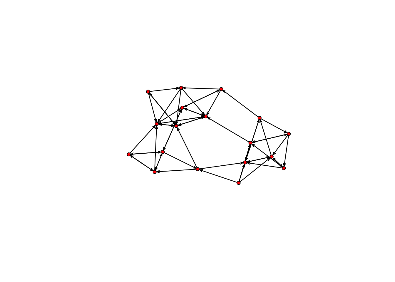

3.4.3.13 Include mutual

sampmodel.01 <- ergm(samplk3~edges+mutual)

## Starting maximum pseudolikelihood estimation (MPLE):

## Evaluating the predictor and response matrix.

## Maximizing the pseudolikelihood.

## Finished MPLE.

## Starting Monte Carlo maximum likelihood estimation (MCMLE):

## Iteration 1 of at most 20:

## Optimizing with step length 1.

## The log-likelihood improved by 0.0002847.

## Step length converged once. Increasing MCMC sample size.

## Iteration 2 of at most 20:

## Optimizing with step length 1.

## The log-likelihood improved by 0.001122.

## Step length converged twice. Stopping.

## Finished MCMLE.

## Evaluating log-likelihood at the estimate. Using 20 bridges: 1 2 3 4 5 6 7 8 9 10 11 12 13 14 15 16 17 18 19 20 .
## This model was fit using MCMC.  To examine model diagnostics and check for degeneracy, use the mcmc.diagnostics() function.

summary(sampmodel.01)

## 
## ==========================
## Summary of model fit
## ==========================
## 
## Formula:   samplk3 ~ edges + mutual
## 
## Iterations:  2 out of 20 
## 
## Monte Carlo MLE Results:
##        Estimate Std. Error MCMC % z value Pr(>|z|)    
## edges   -2.1505     0.2152      0  -9.993   <1e-04 ***
## mutual   2.2849     0.4684      0   4.878   <1e-04 ***
## ---
## Signif. codes:  0 '***' 0.001 '**' 0.01 '*' 0.05 '.' 0.1 ' ' 1
## 
##      Null Deviance: 424.2  on 306  degrees of freedom
##  Residual Deviance: 268.0  on 304  degrees of freedom
##  
## AIC: 272    BIC: 279.5    (Smaller is better.)

Strong mutual effect.

3.4.3.14 Include sender, receiver, mutual

p1 model

sampmodel.02 <- ergm(samplk3~ edges + sender + receiver + mutual)

## Observed statistic(s) receiver10 are at their smallest attainable values. Their coefficients will be fixed at -Inf.

## Starting maximum pseudolikelihood estimation (MPLE):

## Evaluating the predictor and response matrix.

## Maximizing the pseudolikelihood.

## Finished MPLE.

## Starting Monte Carlo maximum likelihood estimation (MCMLE):

## Iteration 1 of at most 20:

## Optimizing with step length 1.

## The log-likelihood improved by 1.081.

## Step length converged once. Increasing MCMC sample size.

## Iteration 2 of at most 20:

## Optimizing with step length 1.

## The log-likelihood improved by 0.08992.

## Step length converged twice. Stopping.

## Finished MCMLE.

## Evaluating log-likelihood at the estimate. Using 20 bridges: 1 2 3 4 5 6 7 8 9 10 11 12 13 14 15 16 17 18 19 20 .
## This model was fit using MCMC.  To examine model diagnostics and check for degeneracy, use the mcmc.diagnostics() function.

summary(sampmodel.02)

## 
## ==========================
## Summary of model fit
## ==========================
## 
## Formula:   samplk3 ~ edges + sender + receiver + mutual
## 
## Iterations:  2 out of 20 
## 
## Monte Carlo MLE Results:
##             Estimate Std. Error MCMC % z value Pr(>|z|)    
## edges      -2.315741   0.796090      0  -2.909  0.00363 ** 
## sender2    -0.438628   1.092996      0  -0.401  0.68819    
## sender3     0.776450   1.093259      0   0.710  0.47757    
## sender4    -0.008577   1.115291      0  -0.008  0.99386    
## sender5    -0.452058   1.134888      0  -0.398  0.69039    
## sender6     0.502989   1.095639      0   0.459  0.64617    
## sender7    -0.252892   1.103350      0  -0.229  0.81871    
## sender8     0.529555   1.111692      0   0.476  0.63382    
## sender9     0.005037   1.122952      0   0.004  0.99642    
## sender10    1.457053   1.055864      0   1.380  0.16760    
## sender11    0.534553   1.100976      0   0.486  0.62730    
## sender12   -0.446945   1.125660      0  -0.397  0.69133    
## sender13    0.530122   1.107423      0   0.479  0.63215    
## sender14    0.529945   1.117297      0   0.474  0.63528    
## sender15    0.508301   1.123175      0   0.453  0.65087    
## sender16    0.793735   1.081730      0   0.734  0.46309    
## sender17    0.526922   1.107444      0   0.476  0.63422    
## sender18    0.235750   1.103263      0   0.214  0.83079    
## receiver2   0.772420   0.896048      0   0.862  0.38867    
## receiver3  -0.739738   0.996962      0  -0.742  0.45809    
## receiver4   0.017002   0.951789      0   0.018  0.98575    
## receiver5   0.766819   0.911852      0   0.841  0.40038    
## receiver6  -1.087262   1.114647      0  -0.975  0.32935    
## receiver7   0.412868   0.901948      0   0.458  0.64713    
## receiver8  -1.111177   1.098415      0  -1.012  0.31172    
## receiver9  -0.001184   0.951954      0  -0.001  0.99901    
## receiver10      -Inf   0.000000      0    -Inf  < 1e-04 ***
## receiver11 -1.089252   1.082136      0  -1.007  0.31414    
## receiver12  0.755936   0.907398      0   0.833  0.40480    
## receiver13 -1.107780   1.098538      0  -1.008  0.31326    
## receiver14 -1.092423   1.110361      0  -0.984  0.32519    
## receiver15 -1.111820   1.099080      0  -1.012  0.31173    
## receiver16 -2.004070   1.347086      0  -1.488  0.13683    
## receiver17 -1.096807   1.109898      0  -0.988  0.32305    
## receiver18 -0.480288   1.012901      0  -0.474  0.63538    
## mutual      3.153694   0.636817      0   4.952  < 1e-04 ***
## ---
## Signif. codes:  0 '***' 0.001 '**' 0.01 '*' 0.05 '.' 0.1 ' ' 1
## 
##      Null Deviance: 424.2  on 306  degrees of freedom
##  Residual Deviance:   NaN  on 270  degrees of freedom
##  
## AIC: NaN    BIC: NaN    (Smaller is better.) 
## 
##  Warning: The following terms have infinite coefficient estimates:
##   receiver10

sna::degree(samplk3,cmode = "indegree")

##  [1] 4 6 3 4 6 2 5 2 4 0 2 6 2 2 2 1 2 3

3.4.3.15 Other ergm-terms

Details of other ergm-terms see https://www.jstatsoft.org/article/view/v024i04.

3.4.4 Missing edges

Make sure to set missing edges as NA: probability of an edge in the observed sample.

missnet=flomarriage
missnet[1,2]=missnet[2,4]=missnet[5,6]=NA # originally are 0
summary(ergm(missnet~edges))

## Starting maximum pseudolikelihood estimation (MPLE):

## Evaluating the predictor and response matrix.

## Maximizing the pseudolikelihood.

## Finished MPLE.

## Stopping at the initial estimate.

## Evaluating log-likelihood at the estimate.

## 
## ==========================
## Summary of model fit
## ==========================
## 
## Formula:   missnet ~ edges
## 
## Iterations:  5 out of 20 
## 
## Monte Carlo MLE Results:
##       Estimate Std. Error MCMC % z value Pr(>|z|)    
## edges  -1.5790     0.2456      0   -6.43   <1e-04 ***
## ---
## Signif. codes:  0 '***' 0.001 '**' 0.01 '*' 0.05 '.' 0.1 ' ' 1
## 
##      Null Deviance: 162.2  on 117  degrees of freedom
##  Residual Deviance: 107.0  on 116  degrees of freedom
##  
## AIC: 109    BIC: 111.8    (Smaller is better.)

summary(ergm(flomarriage~edges))

## Starting maximum pseudolikelihood estimation (MPLE):
## Evaluating the predictor and response matrix.
## Maximizing the pseudolikelihood.
## Finished MPLE.
## Stopping at the initial estimate.
## Evaluating log-likelihood at the estimate.

## 
## ==========================
## Summary of model fit
## ==========================
## 
## Formula:   flomarriage ~ edges
## 
## Iterations:  5 out of 20 
## 
## Monte Carlo MLE Results:
##       Estimate Std. Error MCMC % z value Pr(>|z|)    
## edges  -1.6094     0.2449      0  -6.571   <1e-04 ***
## ---
## Signif. codes:  0 '***' 0.001 '**' 0.01 '*' 0.05 '.' 0.1 ' ' 1
## 
##      Null Deviance: 166.4  on 120  degrees of freedom
##  Residual Deviance: 108.1  on 119  degrees of freedom
##  
## AIC: 110.1    BIC: 112.9    (Smaller is better.)

#Set NA
1/(1+exp(-(-1.5790)))

## [1] 0.1709372

20/(choose(16,2)-3)

## [1] 0.1709402

#Set 0
1/(1+exp(-(-1.6094)))

## [1] 0.1666719

20/(choose(16,2))

## [1] 0.1666667

3.5 simulate netowrks from an ergm model fit

The ergm model defines a probability distibution across all networks of this size(#nodes fixed).

Use simulate(ergm-model,nsim=n) to get a list of networks

Use summary and functions that can be used to a list

summary(flomodel.04)

## 
## ==========================
## Summary of model fit
## ==========================
## 
## Formula:   flomarriage ~ edges + absdiff("wealth")
## 
## Iterations:  4 out of 20 
## 
## Monte Carlo MLE Results:
##                 Estimate Std. Error MCMC % z value Pr(>|z|)    
## edges          -2.302042   0.401906      0  -5.728   <1e-04 ***
## absdiff.wealth  0.015519   0.006157      0   2.521   0.0117 *  
## ---
## Signif. codes:  0 '***' 0.001 '**' 0.01 '*' 0.05 '.' 0.1 ' ' 1
## 
##      Null Deviance: 166.4  on 120  degrees of freedom
##  Residual Deviance: 102.0  on 118  degrees of freedom
##  
## AIC: 106    BIC: 111.5    (Smaller is better.)

flomodel.04.sim <- simulate(flomodel.04, nsim=10,seed = 1)

## Warning: You appear to be calling simulate.formula() directly.
## simulate.formula() is a method, and will not be exported in a future
## version of 'ergm'. Use simulate() instead, or getS3method() if absolutely
## necessary.

class(flomodel.04.sim)

## [1] "network.list"

summary(flomodel.04.sim)

## Number of Networks: 10 
## Model: flomarriage ~ edges + absdiff("wealth") 
## Reference: ~Bernoulli 
## Constraints: ~. 
## Parameters:
##          edges absdiff.wealth 
##     -2.3020421      0.0155192 
## 
## Stored network statistics:
##       edges absdiff.wealth
##  [1,]    20           1070
##  [2,]    22           1170
##  [3,]    19            734
##  [4,]    18           1123
##  [5,]    18           1215
##  [6,]    15            697
##  [7,]    20           1165
##  [8,]    31           1577
##  [9,]    19           1138
## [10,]    22           1136

## Number of Networks: 10 
## Model: flomarriage ~ edges + absdiff("wealth") 
## Reference: ~Bernoulli 
## Constraints: ~. 
## Parameters:
##          edges absdiff.wealth 
##     -2.3020421      0.0155192

length(flomodel.04.sim)

## [1] 10

flomodel.04.sim[[4]]

##  Network attributes:
##   vertices = 16 
##   directed = FALSE 
##   hyper = FALSE 
##   loops = FALSE 
##   multiple = FALSE 
##   bipartite = FALSE 
##   total edges= 18 
##     missing edges= 0 
##     non-missing edges= 18 
## 
##  Vertex attribute names: 
##     priorates totalties vertex.names wealth 
## 
## No edge attributes

plot(flomodel.04.sim[[4]], label= flomodel.04.sim[[4]] %v% "vertex.names")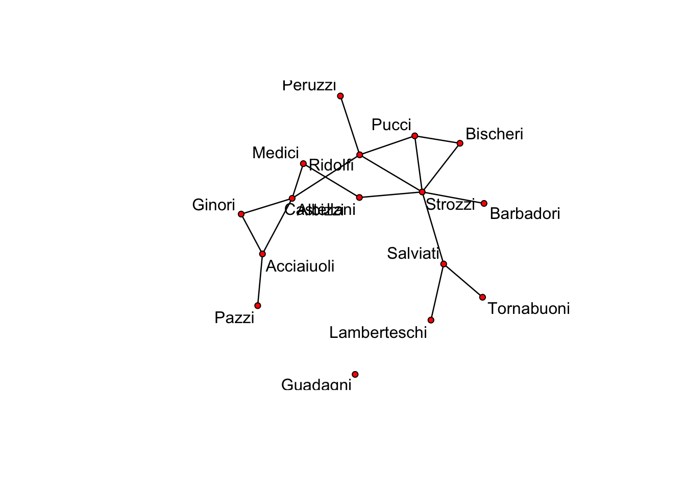

flomarriage

##  Network attributes:
##   vertices = 16 
##   directed = FALSE 
##   hyper = FALSE 
##   loops = FALSE 
##   multiple = FALSE 
##   bipartite = FALSE 
##   total edges= 20 
##     missing edges= 0 
##     non-missing edges= 20 
## 
##  Vertex attribute names: 
##     priorates totalties vertex.names wealth 
## 
## No edge attributes

---

• formula: Specify your own model

• basis: initial network for MC

• control: settings of MCMC

basenet <- network(16,density=0.1,directed=FALSE)
g.sim <- simulate(flomarriage ~ edges + kstar(2), nsim=1000, coef=c(-1.8,0.03),
                  basis=basenet, control=control.simulate(MCMC.burnin=1000, MCMC.interval=10))
# MCMC.interval: Number of proposals between sampled statistics. 
length(g.sim)

## [1] 1000

?simulate.ergm

3.6 Check the goodness of fit

• AIC,BIC; Deviance;
• Goodness of fit: gof
• MCMC diagnostics: mcmc.diagnostics

3.6.1 gof

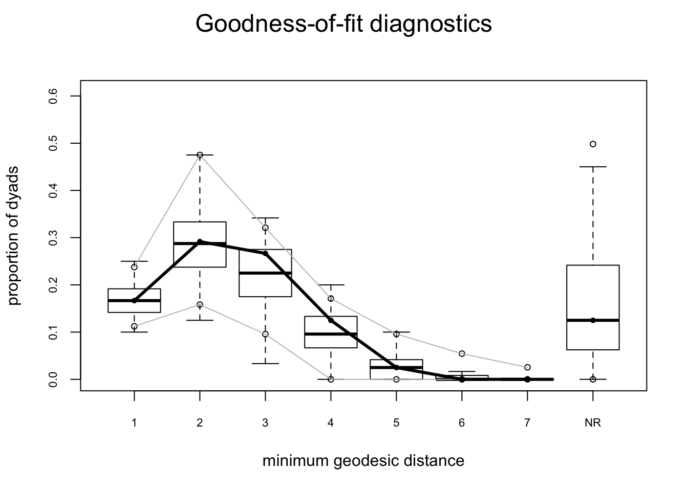
gof(model~model+degree+esp+distance)

Only four possible arguments for ergm-term:

• model: all the terms included in the model
• degree: degree (node level)
• esp: edgwise share partners (edge level)
• distance: geodesic distances (dyad level)

Draw samples from the specified model, calculate the MC p-value based on the distribution generated by the samples.

flo.04.gof.model=gof(flomodel.04~model+degree+esp+distance)
flo.04.gof.model

## 
## Goodness-of-fit for model statistics 
## 
##                 obs min    mean  max MC p-value
## edges            20  12   20.22   30       1.00
## absdiff.wealth 1146 565 1142.44 1841       0.96
## 
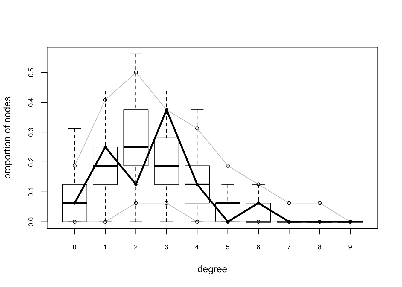
## Goodness-of-fit for degree 
## 
##    obs min mean max MC p-value
## 0    1   0 1.24   5       1.00
## 1    4   0 3.15   8       0.74
## 2    2   0 4.51   9       0.24
## 3    6   0 3.32   7       0.18
## 4    2   0 2.01   6       1.00
## 5    0   0 0.91   4       0.72
## 6    1   0 0.50   3       0.82
## 7    0   0 0.22   2       1.00
## 8    0   0 0.10   1       1.00
## 9    0   0 0.02   1       1.00
## 10   0   0 0.02   1       1.00
## 
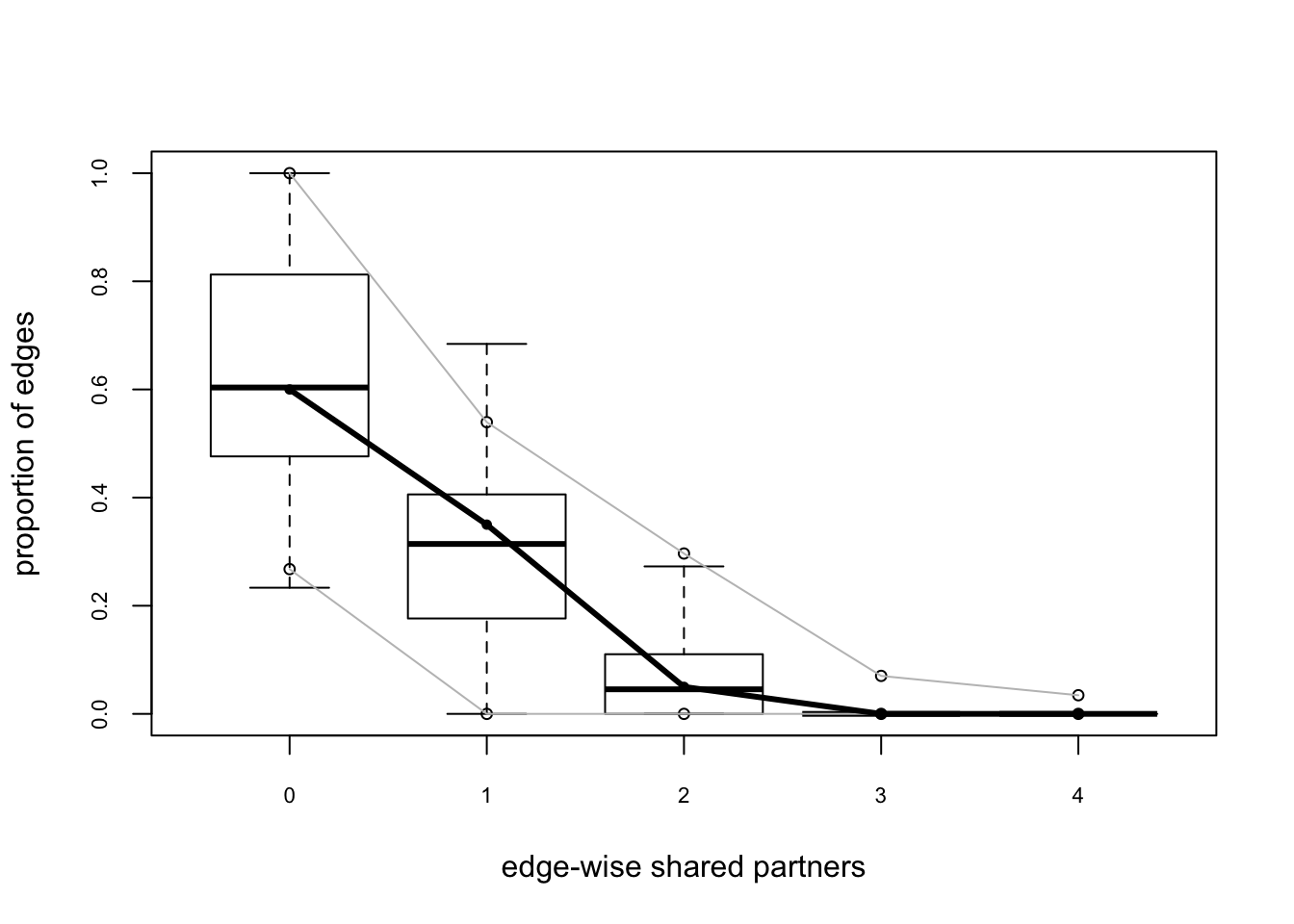
## Goodness-of-fit for edgewise shared partner 
## 
##      obs min  mean max MC p-value
## esp0  12   5 12.39  23       1.00
## esp1   7   0  5.99  14       0.94
## esp2   1   0  1.60  12       1.00
## esp3   0   0  0.19   4       1.00
## esp4   0   0  0.05   1       1.00
## 
## Goodness-of-fit for minimum geodesic distance 
## 
##     obs min  mean max MC p-value
## 1    20  12 20.22  30       1.00
## 2    35  15 35.01  58       1.00
## 3    32   4 26.70  41       0.58
## 4    15   0 11.11  24       0.60
## 5     3   0  3.35  14       1.00
## 6     0   0  0.89  11       1.00
## 7     0   0  0.21   6       1.00
## 8     0   0  0.06   3       1.00
## 9     0   0  0.02   2       1.00
## Inf  15   0 22.43  73       1.00

names(flo.04.gof.model)

##  [1] "network.size"   "GOF"            "pval.model"     "summary.model" 
##  [5] "pobs.model"     "psim.model"     "bds.model"      "obs.model"     
##  [9] "sim.model"      "pval.dist"      "summary.dist"   "pobs.dist"     
## [13] "psim.dist"      "bds.dist"       "obs.dist"       "sim.dist"      
## [17] "pval.deg"       "summary.deg"    "pobs.deg"       "psim.deg"      
## [21] "bds.deg"        "obs.deg"        "sim.deg"        "pval.espart"   
## [25] "summary.espart" "pobs.espart"    "psim.espart"    "bds.espart"    
## [29] "obs.espart"     "sim.espart"

#95% confidence interval
plot(flo.04.gof.model)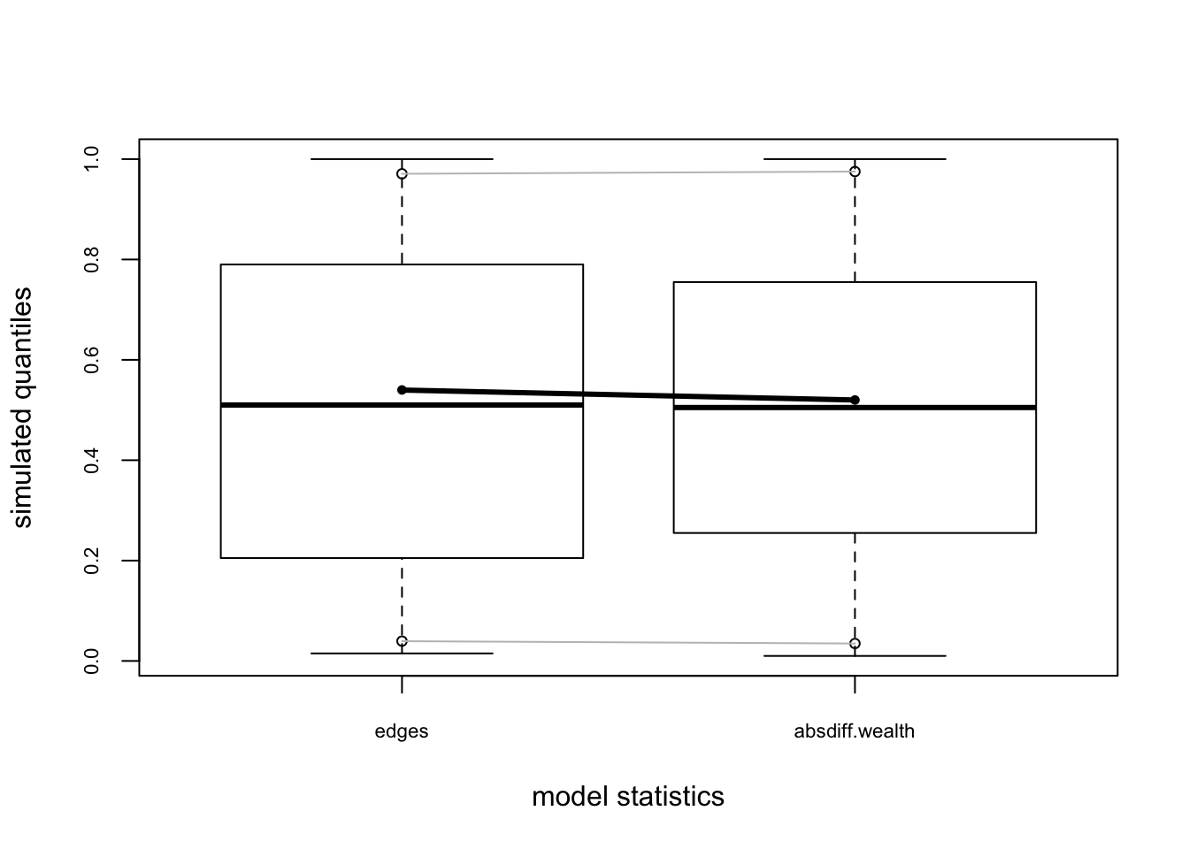

3.6.2 mcmc.diagnostics

Check the MCMC

#install.packages("latticeExtra")

fit <- ergm(flobusiness ~ edges+degree(1))

## Starting maximum pseudolikelihood estimation (MPLE):

## Evaluating the predictor and response matrix.

## Maximizing the pseudolikelihood.

## Finished MPLE.

## Starting Monte Carlo maximum likelihood estimation (MCMLE):

## Iteration 1 of at most 20:

## Optimizing with step length 1.

## The log-likelihood improved by 0.2425.

## Step length converged once. Increasing MCMC sample size.

## Iteration 2 of at most 20:

## Optimizing with step length 1.

## The log-likelihood improved by 0.001113.

## Step length converged twice. Stopping.

## Finished MCMLE.

## Evaluating log-likelihood at the estimate. Using 20 bridges: 1 2 3 4 5 6 7 8 9 10 11 12 13 14 15 16 17 18 19 20 .
## This model was fit using MCMC.  To examine model diagnostics and check for degeneracy, use the mcmc.diagnostics() function.

mcmc.diagnostics(fit) #centered

## Sample statistics summary:
## 
## Iterations = 16384:4209664
## Thinning interval = 1024 
## Number of chains = 1 
## Sample size per chain = 4096 
## 
## 1. Empirical mean and standard deviation for each variable,
##    plus standard error of the mean:
## 
##             Mean    SD Naive SE Time-series SE
## edges   -0.12183 3.766  0.05884        0.05884
## degree1  0.07349 1.634  0.02553        0.02553
## 
## 2. Quantiles for each variable:
## 
##         2.5% 25% 50% 75% 97.5%
## edges     -7  -3   0   2     7
## degree1   -4  -1   0   1     3
## 
## 
## Sample statistics cross-correlations:
##           edges degree1
## edges    1.0000 -0.4341
## degree1 -0.4341  1.0000
## 
## Sample statistics auto-correlation:
## Chain 1 
##                 edges      degree1
## Lag 0     1.000000000  1.000000000
## Lag 1024  0.006760343  0.001466041
## Lag 2048  0.008602875 -0.006057681
## Lag 3072 -0.018218817 -0.011568388
## Lag 4096  0.028773889 -0.015764465
## Lag 5120 -0.015302900 -0.004412151
## 
## Sample statistics burn-in diagnostic (Geweke):
## Chain 1 
## 
## Fraction in 1st window = 0.1
## Fraction in 2nd window = 0.5 
## 
##   edges degree1 
##  0.9156 -0.5825 
## 
## Individual P-values (lower = worse):
##     edges   degree1 
## 0.3598522 0.5602179 
## Joint P-value (lower = worse):  0.6503828 .

## Warning in formals(fun): argument is not a function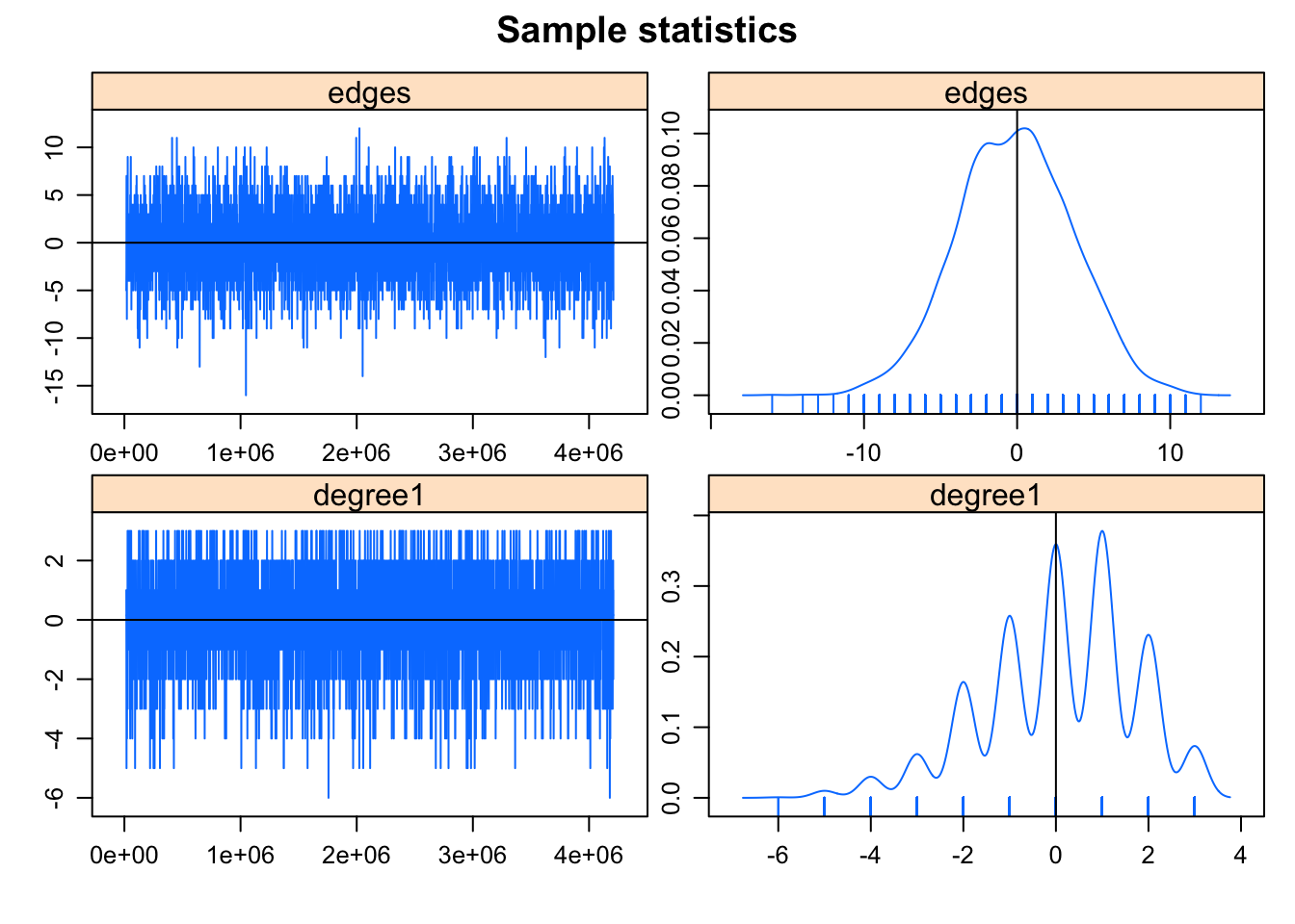

## 
## MCMC diagnostics shown here are from the last round of simulation, prior to computation of final parameter estimates. Because the final estimates are refinements of those used for this simulation run, these diagnostics may understate model performance. To directly assess the performance of the final model on in-model statistics, please use the GOF command: gof(ergmFitObject, GOF=~model).

---

Interpretation on mcmc.diagnostics:

Good example.

• Mixing well: MCMC sample statistics are varying randomly around the observed values at each step
• Bell-shaped centered at 0. The difference between the observed and simulated values of the sample statistics have a roughly bell-shaped distribution, centered at 0.
• Notice the sawtooth pattern is due to the discrete values. The sawtooth pattern visible on the degree term deviation plot is due to the combination of discrete values and small range in the statistics: the observed number of degree 1 nodes is 3, and only a few discrete values are produced by the simulations.

Bad example:

Figure 3.1: Example from Tutorial

3.7 More functions

Figure 3.2: Example from Tutorial