SLR: Simulation based-inference

STA 210 - Summer 2022

Author

Yunran Chen

Welcome

Announcements

HW 1 posted on Monday, due Wednesday, May 18, 11:59pm.
Lab 2 posted on Monday, due Friday, May 20, 11:59pm.
AE 2 posted on Monday, due Wednesday, May 18, 11:59pm.

Tips for collaboration on Github

Frustrating, but part of our goal for the class
Widely-used for version control and collaboration
Merge issue

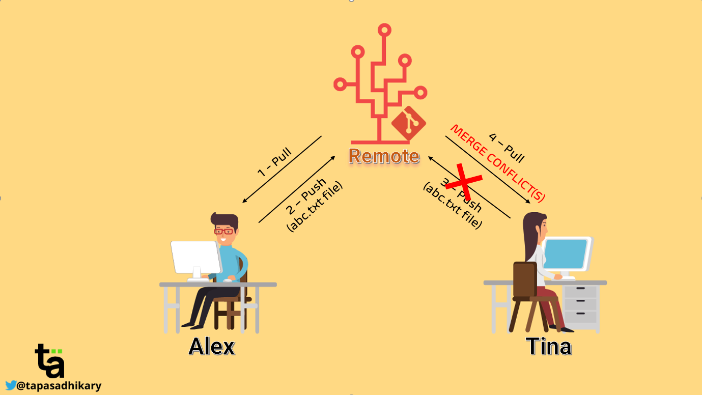
Merge Issue on Github

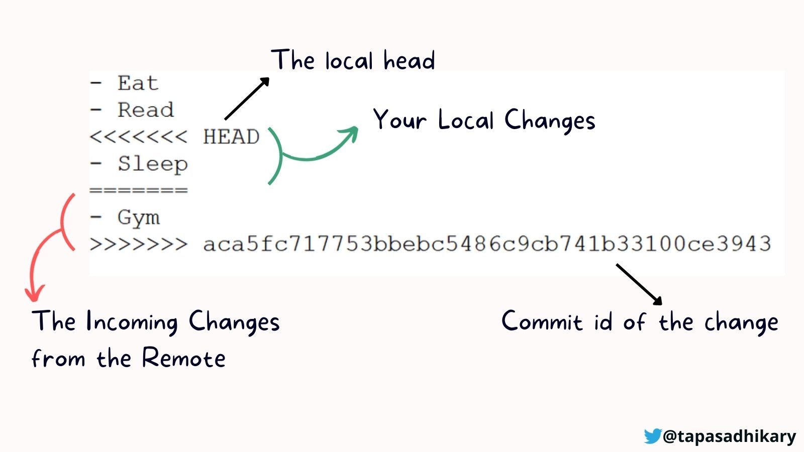Github merge issues ## Merge Issue on Github

Having merge issue: pull - re-edit, merge issue - commit - push
To avoid merge conflicts:
- Work on different parts of the lab. Do not edit the same part simultaneously.
- Create your own rmd file using your own name, and only edit your file. Then merge all changes.
- Always pull before you start any new logical work on your code.
- Talk to your team members when you need to make changes related to their part

Computational setup

# load packages
library(tidyverse)   # for data wrangling and visualization
library(tidymodels)  # for modeling
library(usdata)      # for the county_2019 dataset
library(openintro)   # for the duke_forest dataset
library(scales)      # for pretty axis labels
library(glue)        # for constructing character strings
library(knitr)       # for pretty tables

# set default theme and larger font size for ggplot2
ggplot2::theme_set(ggplot2::theme_minimal(base_size = 16))

Recap of last lecture

Terminology

Outcome: y
Predictor: x
Observed y, $y$: truth
Predicted y, $\hat{y}$: fitted, estimated
Residual: $y-\hat{y}$

Model evaluation

Evaluating models’ performance for fitting
- R-squared, RMSE
Interested in performance for prediction for a new observation
Evaluating predictive performance: Splitting the data
Quantifying variability of of estimates: Bootstrap the data

Model evaluation

Evaluating predictive performance: Split the data into testing and training sets, build models using only the training set, and evaluate their performance on the testing set, and repeat to see how your model holds up to “new” data
Quantifying variability of of estimates: Bootstrap the data, fit a model, obtain coefficient estimates and/or measures of strength of fit, and repeat many times to see how your model holds up to “new” data

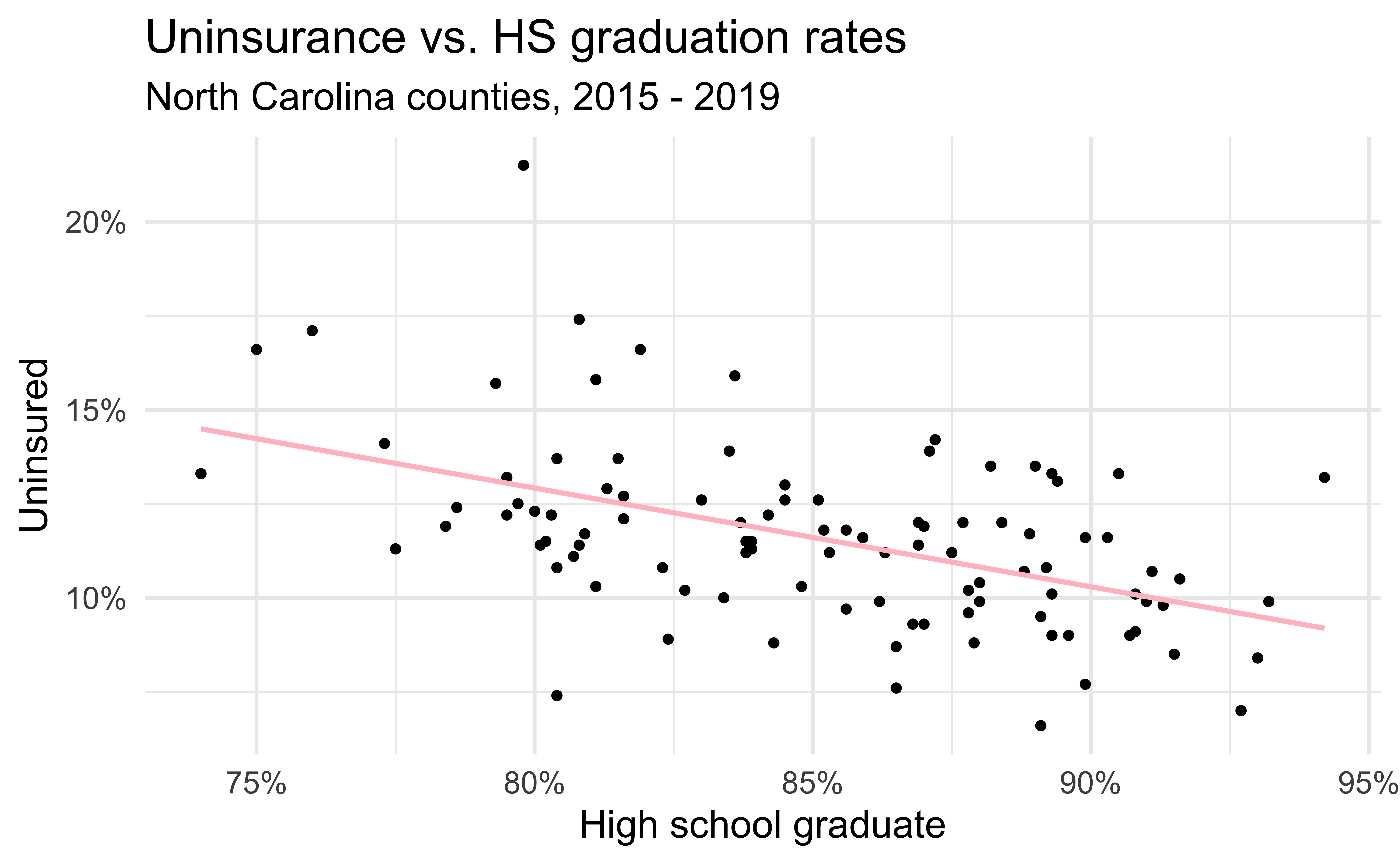
Uninsurance vs. HS graduation in NC

Uninsurance vs. HS graduation in NY

Code

county_2019_ny <- county_2019 %>%
  as_tibble() %>%
  filter(state == "New York") %>%
  select(name, hs_grad, uninsured)

ggplot(county_2019_ny,
       aes(x = hs_grad, y = uninsured)) +
  geom_point() +
  scale_x_continuous(labels = label_percent(scale = 1, accuracy = 1)) +
  scale_y_continuous(labels = label_percent(scale = 1, accuracy = 1)) +
  labs(
    x = "High school graduate", y = "Uninsured",
    title = "Uninsurance vs. HS graduation rates",
    subtitle = "New York counties, 2015 - 2019"
  ) +
  geom_smooth(method = "lm", se = FALSE, color = "pink")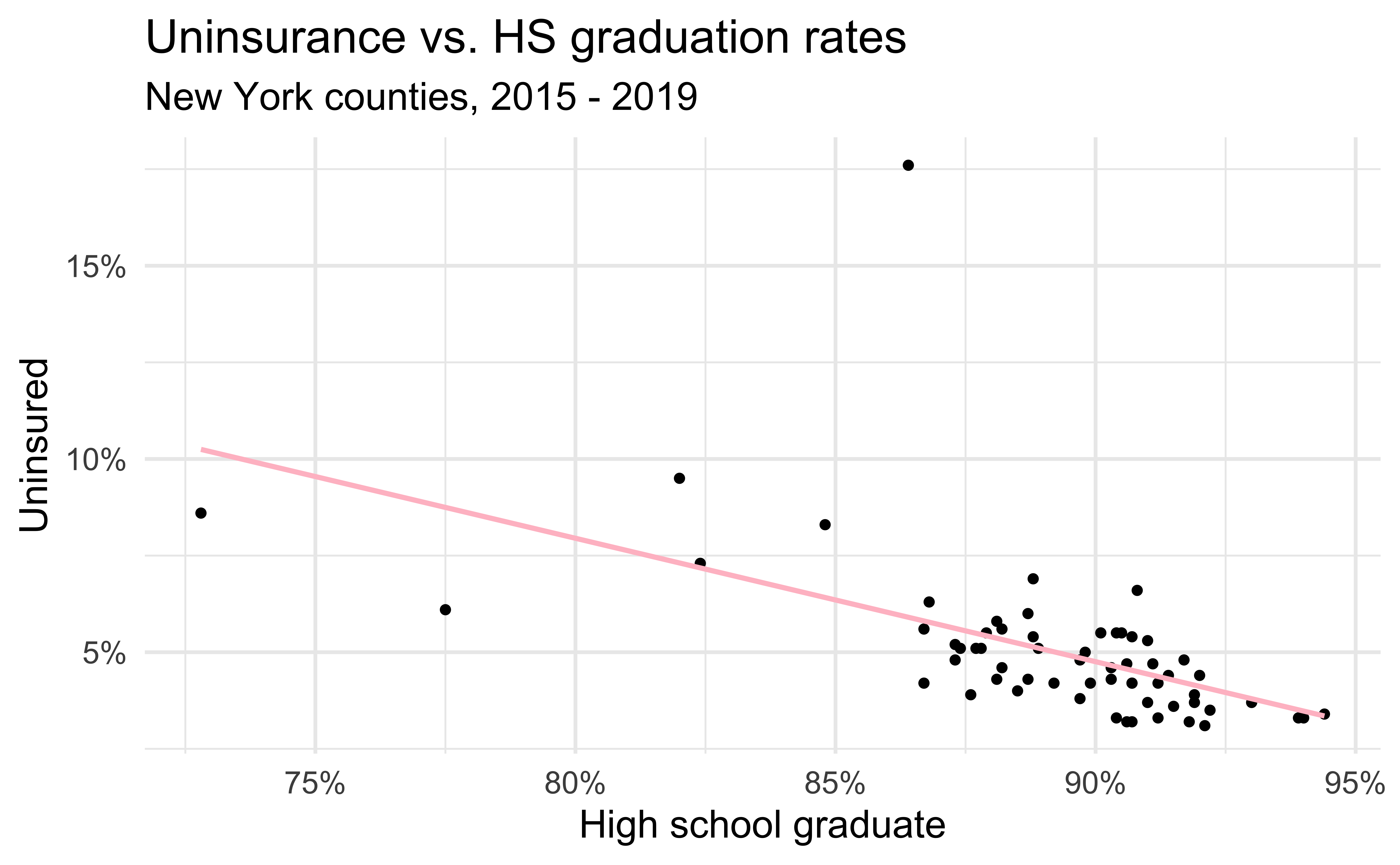

Data splitting

Bootstrapping

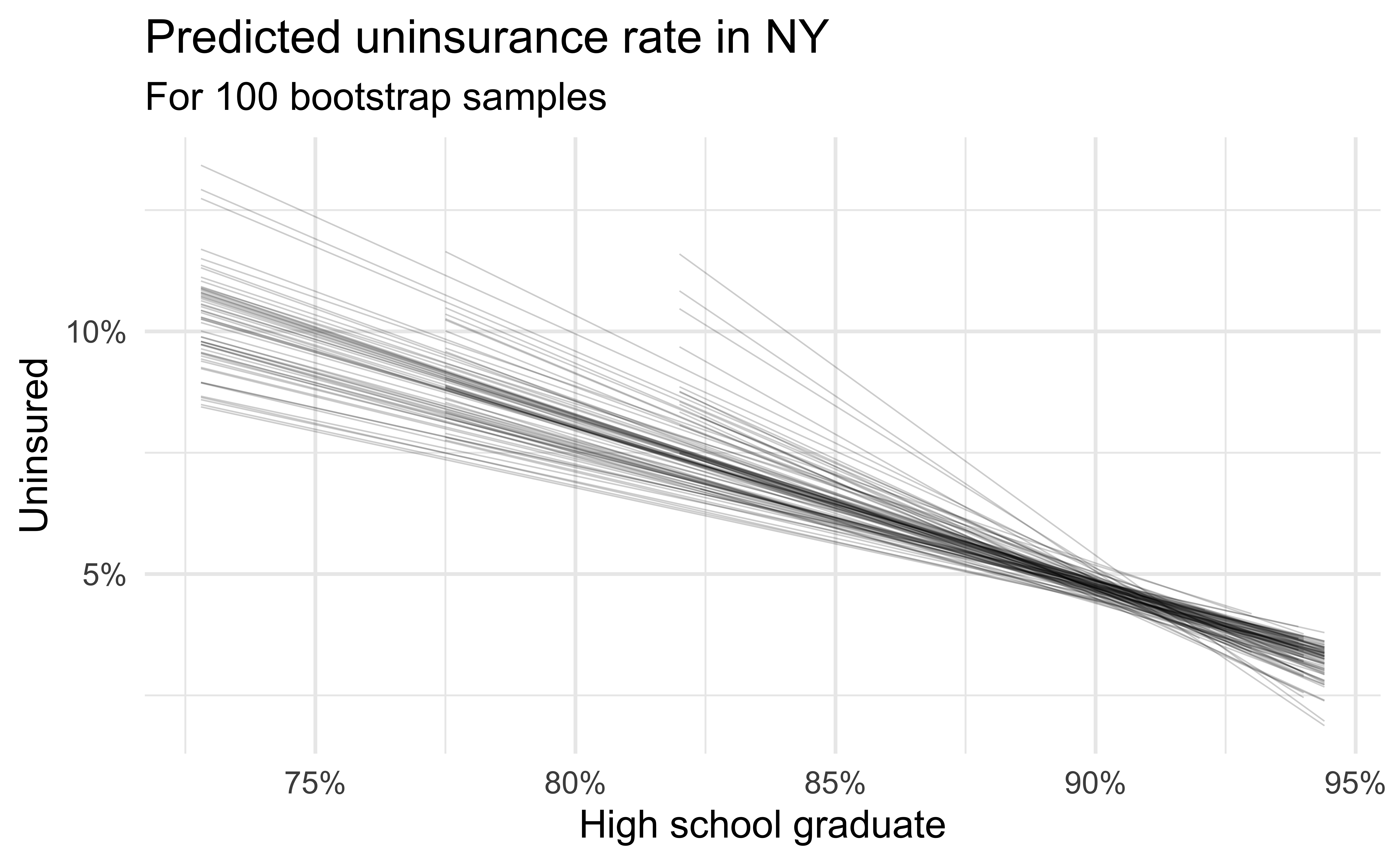
Comparing NY and NC

Why are the fits from the NY models more variable than those from the NC models?

Sample size
Outliers or influential points

Statistical inference

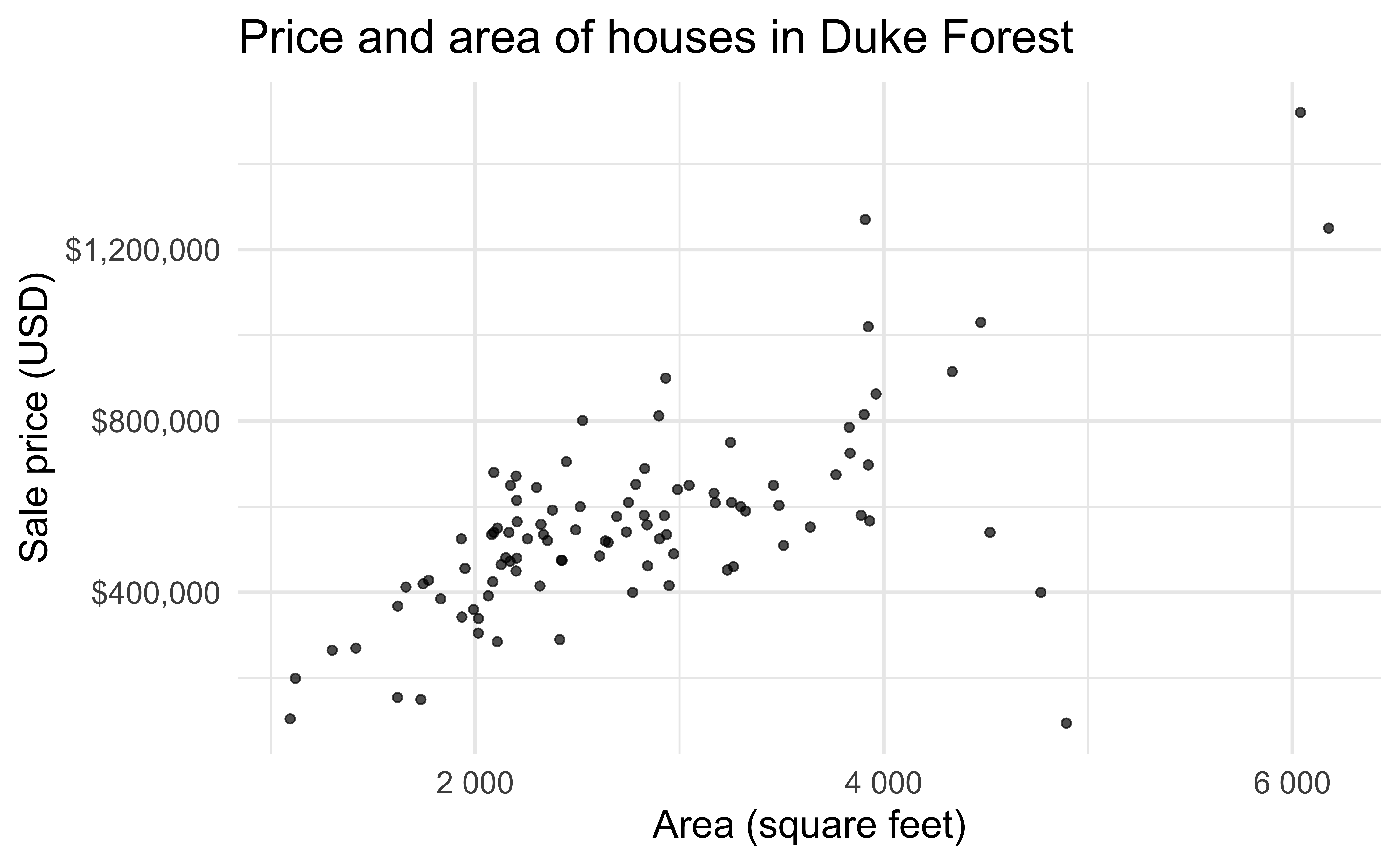
Data: Sale prices of houses in Duke Forest

Data on houses that were sold in the Duke Forest neighborhood of Durham, NC around November 2020
Scraped from Zillow
Source: openintro::duke_forest

Exploratory analysis

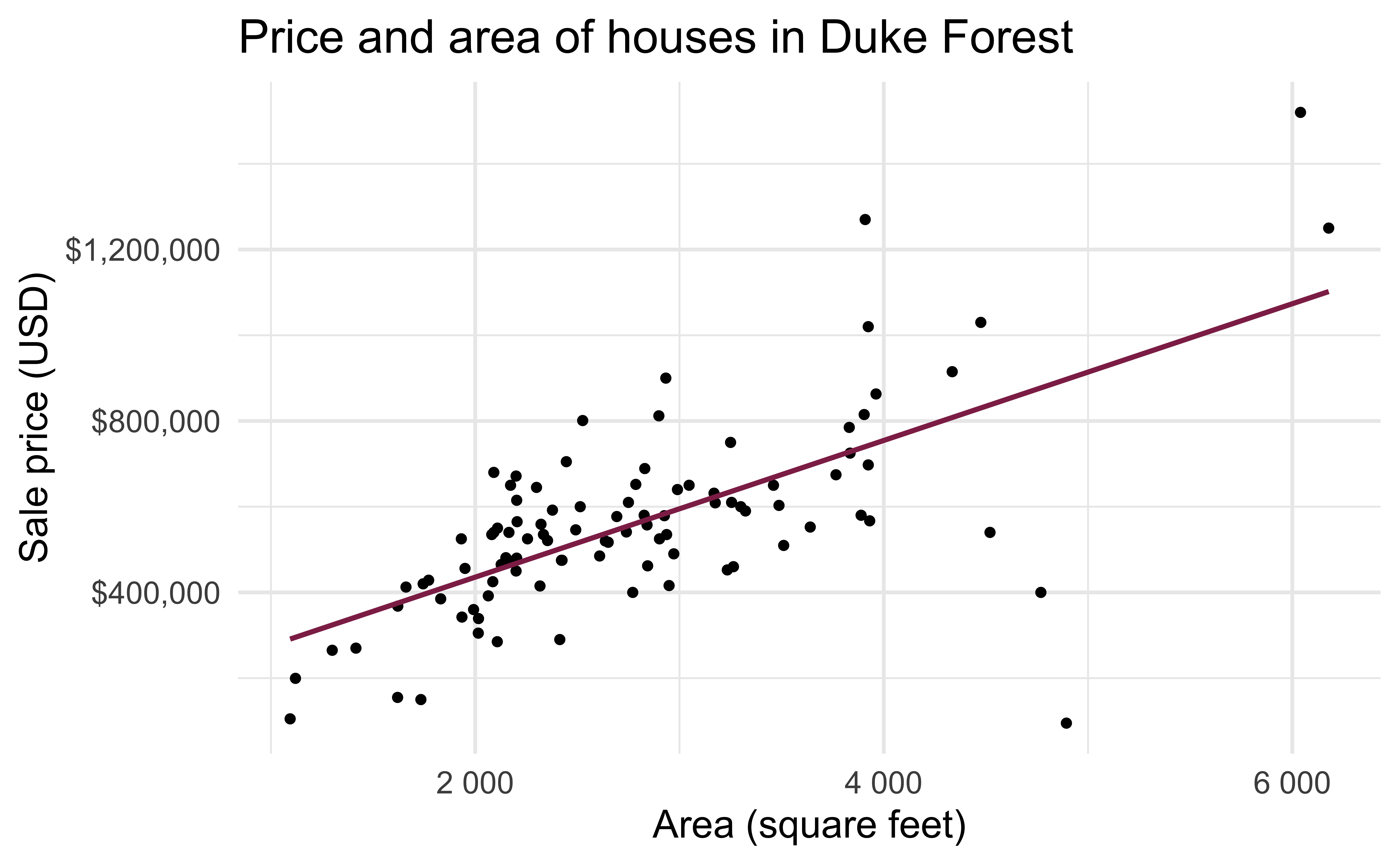
Modeling

df_fit <- linear_reg() %>%
  set_engine("lm") %>%
  fit(price ~ area, data = duke_forest)

tidy(df_fit) %>%
  kable(digits = 2)

term	estimate	std.error	statistic	p.value
(Intercept)	116652.33	53302.46	2.19	0.03
area	159.48	18.17	8.78	0.00

Intercept: Duke Forest houses that are 0 square feet are expected to sell, on average, for $116,652.
Slope: For each additional square foot, the model predicts (we expect) the sale price of Duke Forest houses to be higher, on average, by $159.

Sample to population

For each additional square foot, the model predicts the sale price of Duke Forest houses to be higher, on average, by $159.

This estimate is valid for the single sample of 98 houses.
But what if we’re not interested quantifying the relationship between the size and price of a house in this single sample?
What if we want to say something about the relationship between these variables for all houses in Duke Forest?

Statistical inference

Statistical inference allows provide methods and tools for us to use the single sample we have observed to make valid statements (inferences) about the population it comes from
For our inferences to be valid, the sample should be random and representative of the population we’re interested in

Inference for simple linear regression

Calculate a confidence interval for the slope, $\beta_1$
Conduct a hypothesis test for the slope, $\beta_1$

Confidence interval for the slope

Confidence interval

A plausible range of values for a population parameter is called a confidence interval
Using only a single point estimate is like fishing in a murky lake with a spear, and using a confidence interval is like fishing with a net
- We can throw a spear where we saw a fish but we will probably miss, if we toss a net in that area, we have a good chance of catching the fish
- Similarly, if we report a point estimate, we probably will not hit the exact population parameter, but if we report a range of plausible values we have a good shot at capturing the parameter

Confidence interval for the slope

A confidence interval will allow us to make a statement like “For each additional square foot, the model predicts the sale price of Duke Forest houses to be higher, on average, by $159, give or take X dollars.”

Should X be $10? $100? $1000? (width of interval)
If we were to take another sample of 98 would we expect the slope calculated based on that sample to be exactly $159? Off by $10? $100? $1000?
The answer depends on how variable (from one sample to another sample) the sample statistic (the slope) is
We need a way to quantify the variability of the sample statistic

Quantify the variability of the slope

for estimation

Two approaches:
1. Via simulation (what we’ll do today)
2. Via mathematical models (what we’ll do in the next class)
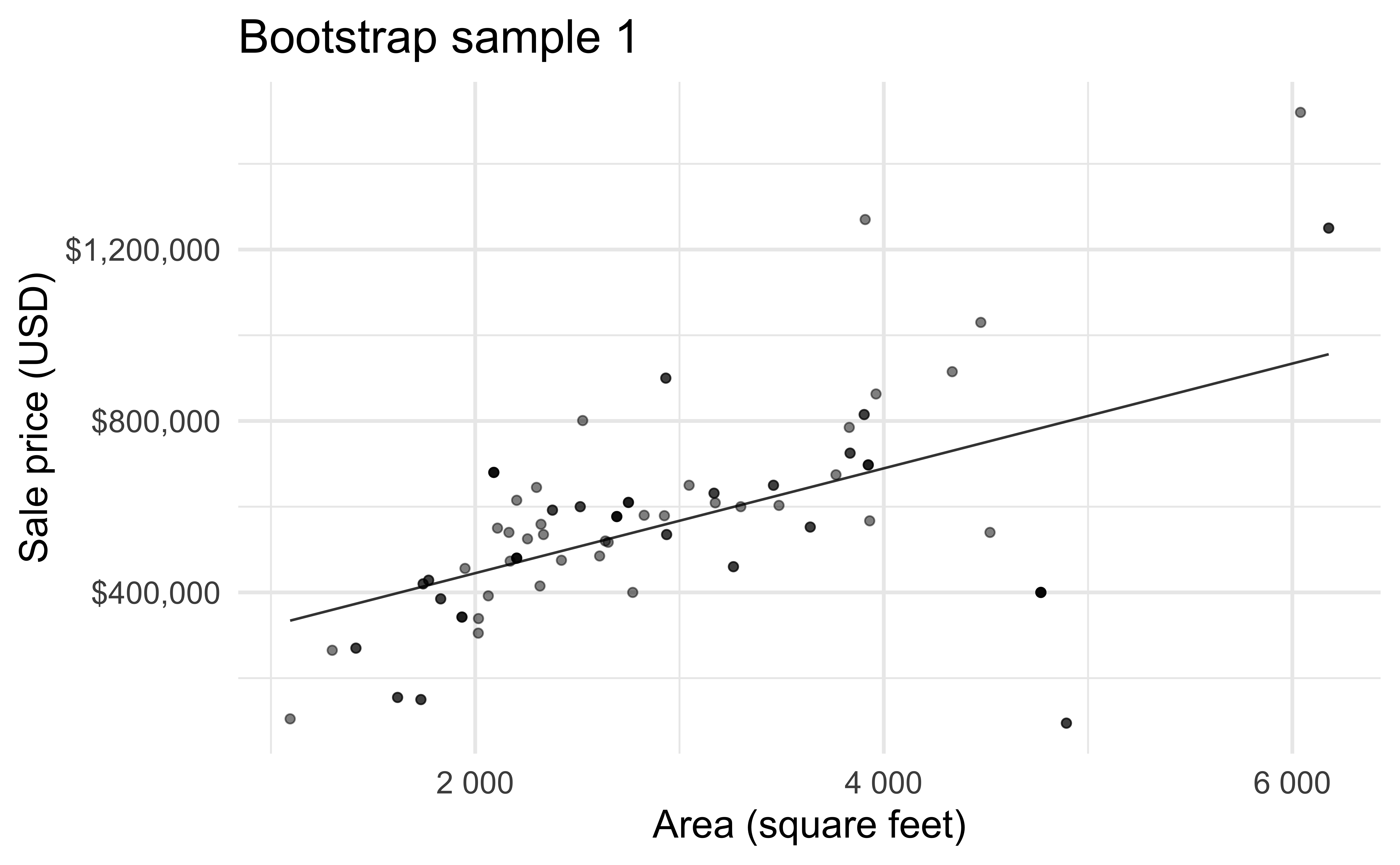
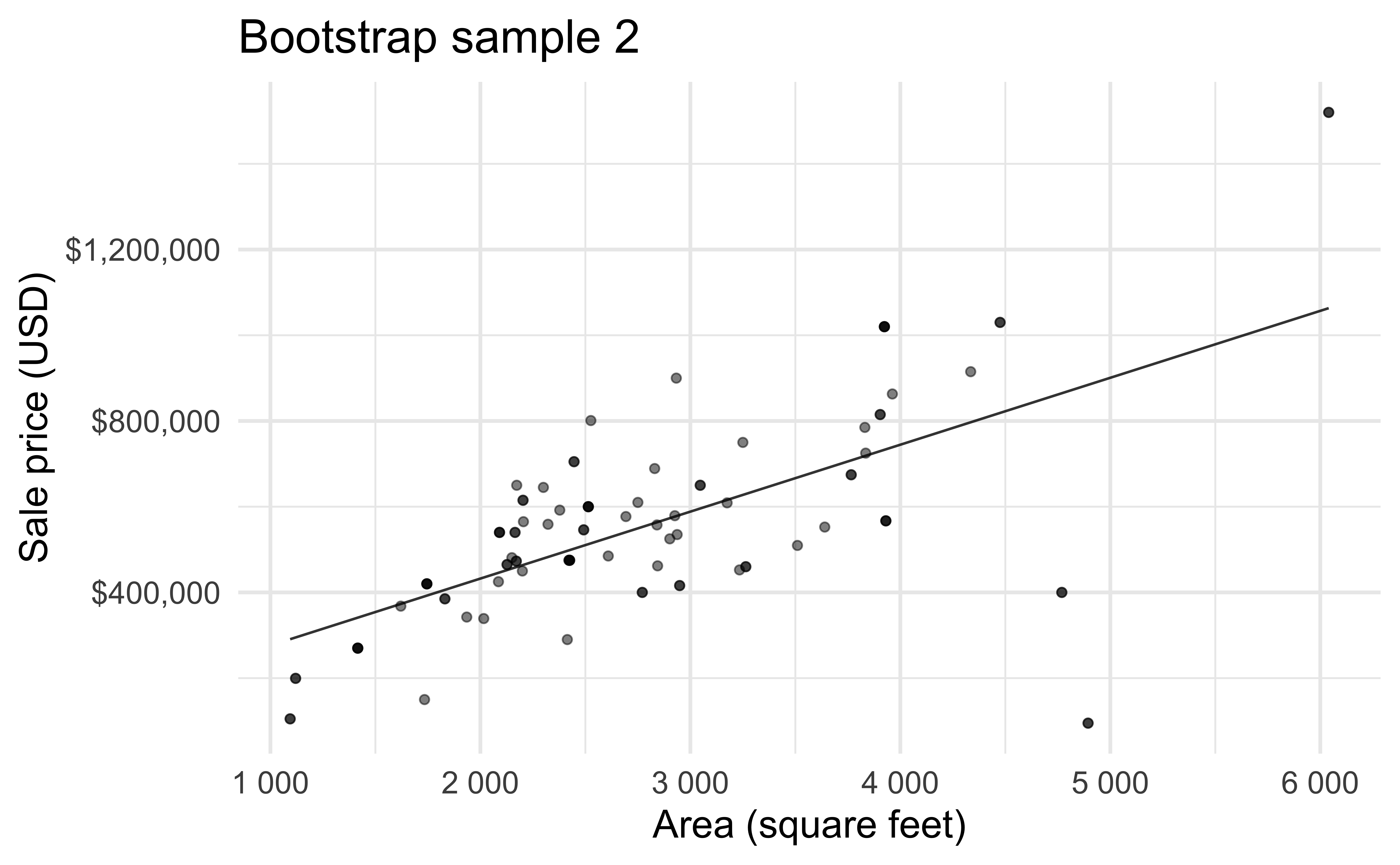
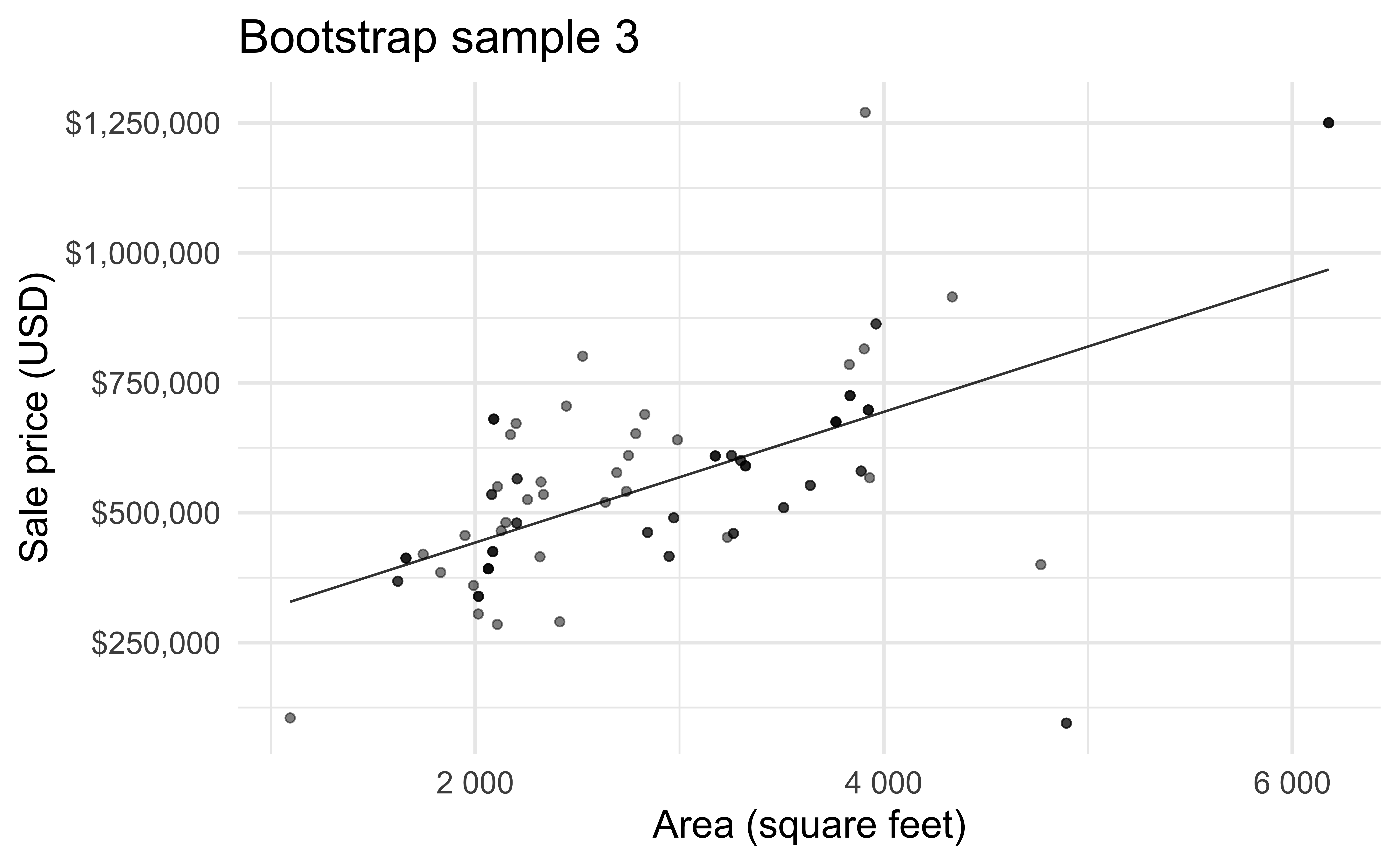
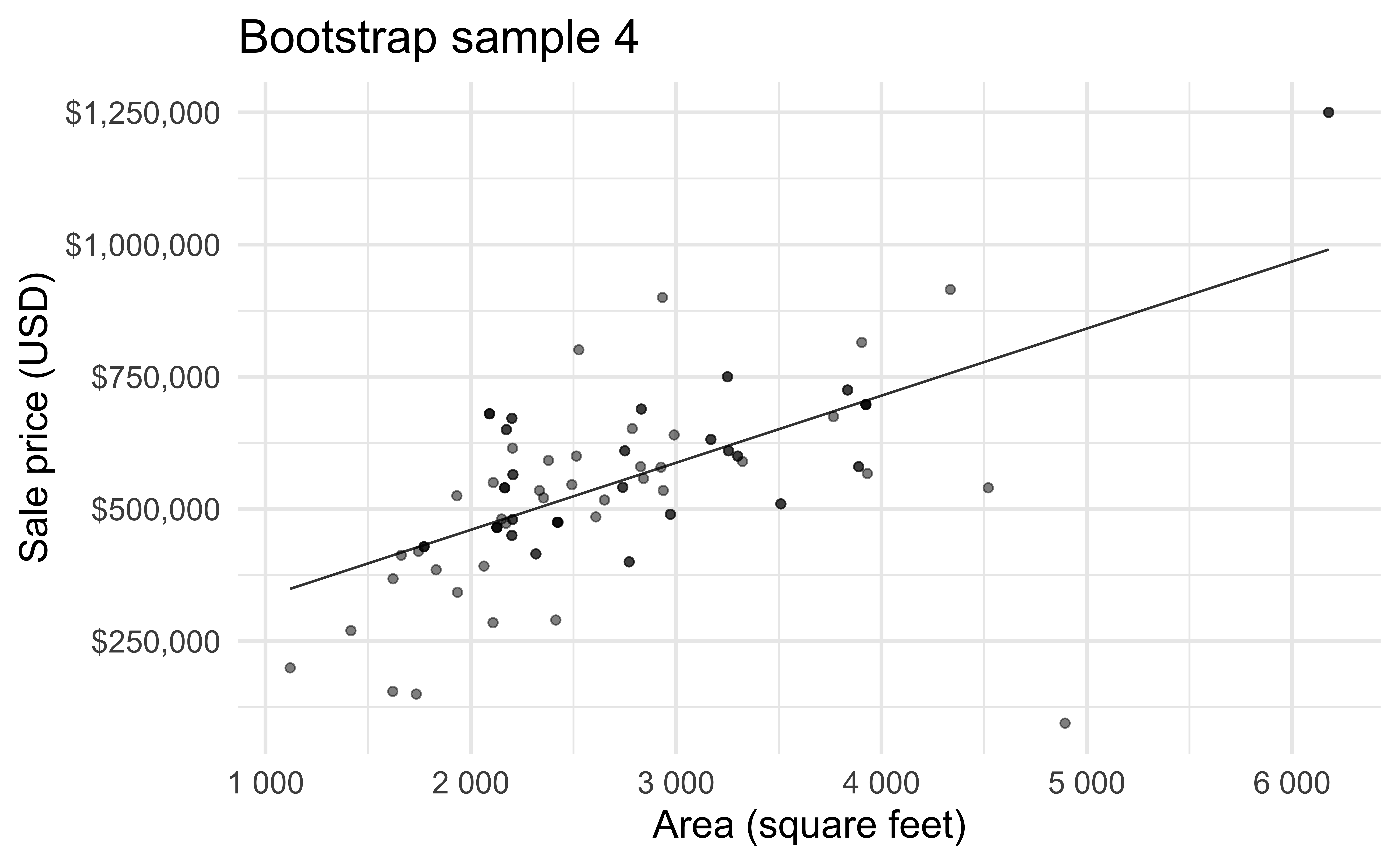
Bootstrapping to quantify the variability of the slope for the purpose of estimation:
- Bootstrap new samples from the original sample
- Fit models to each of the samples and estimate the slope
- Use features of the distribution of the bootstrapped slopes to construct a confidence interval

Bootstrap sample 1

Bootstrap sample 2

Bootstrap sample 3

Bootstrap sample 4

Bootstrap sample 5

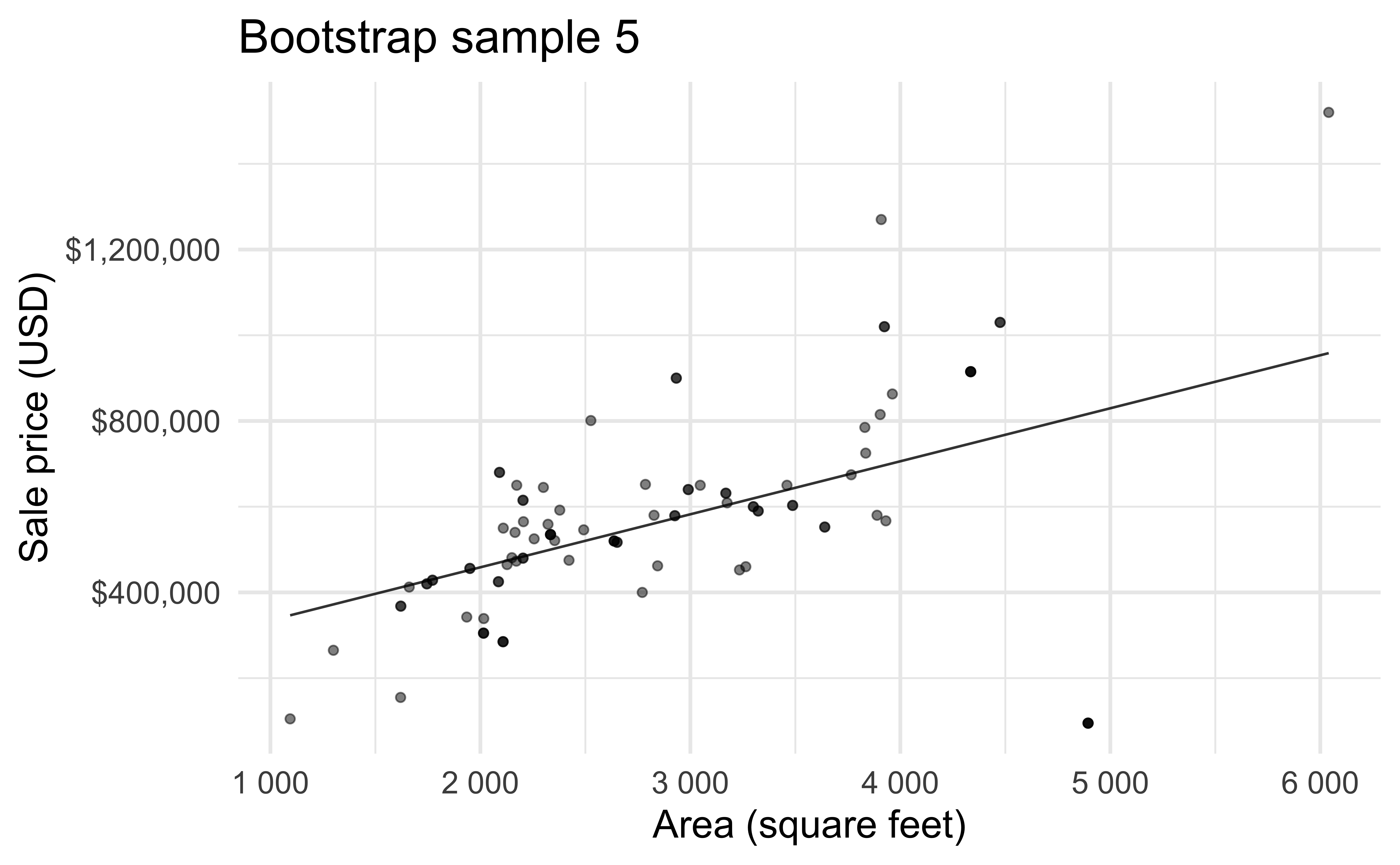
so on and so forth…

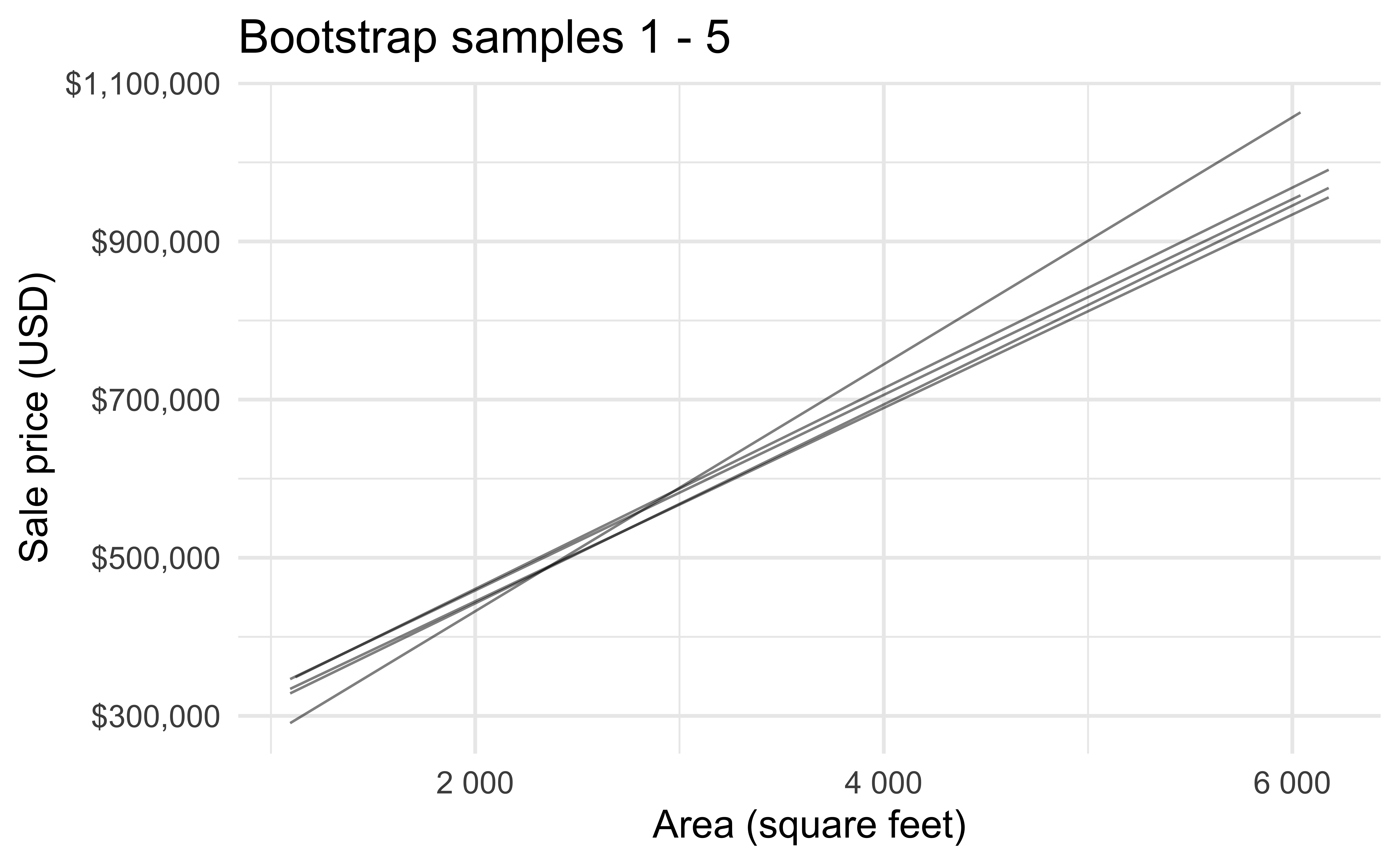
Bootstrap samples 1 - 5

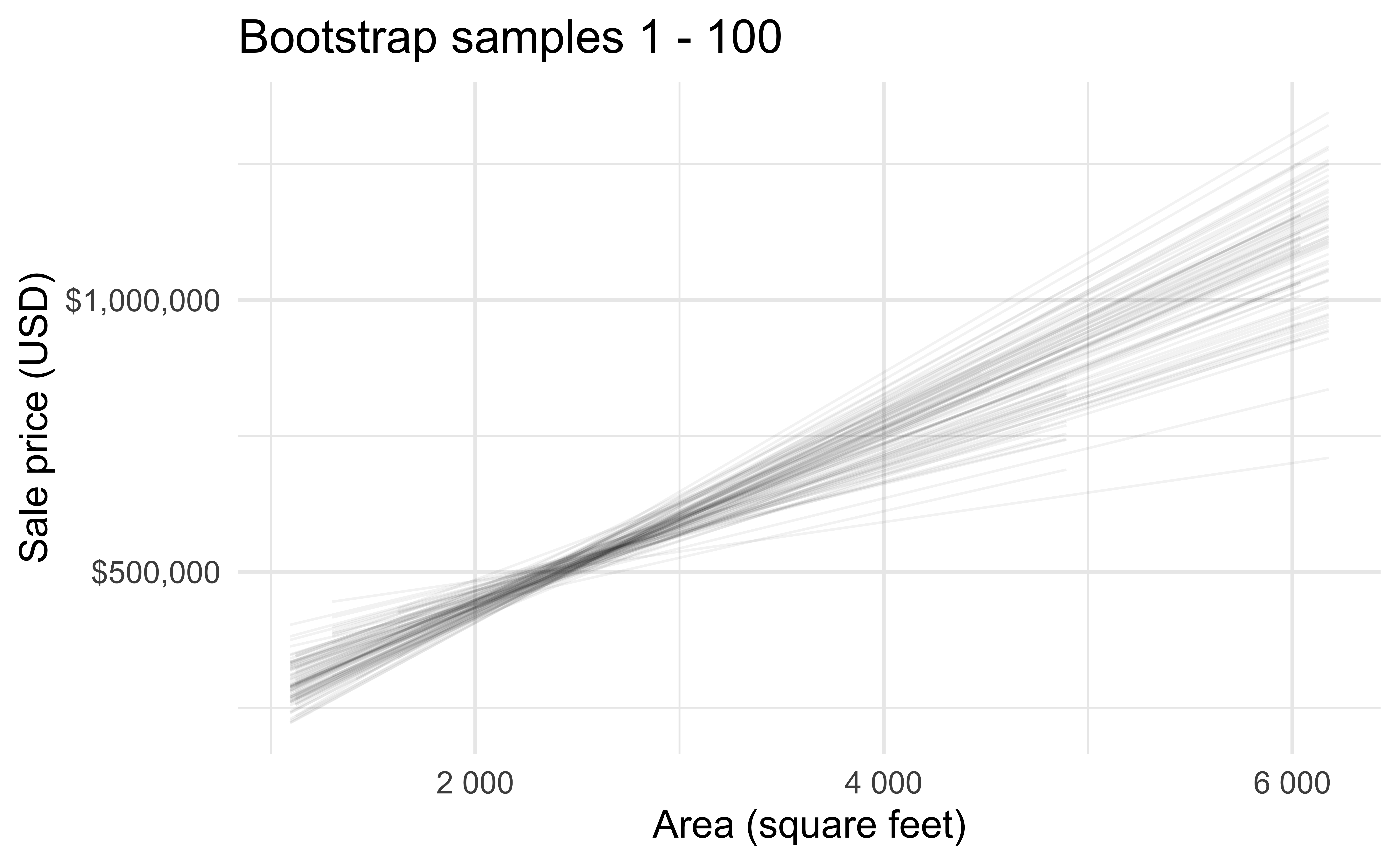
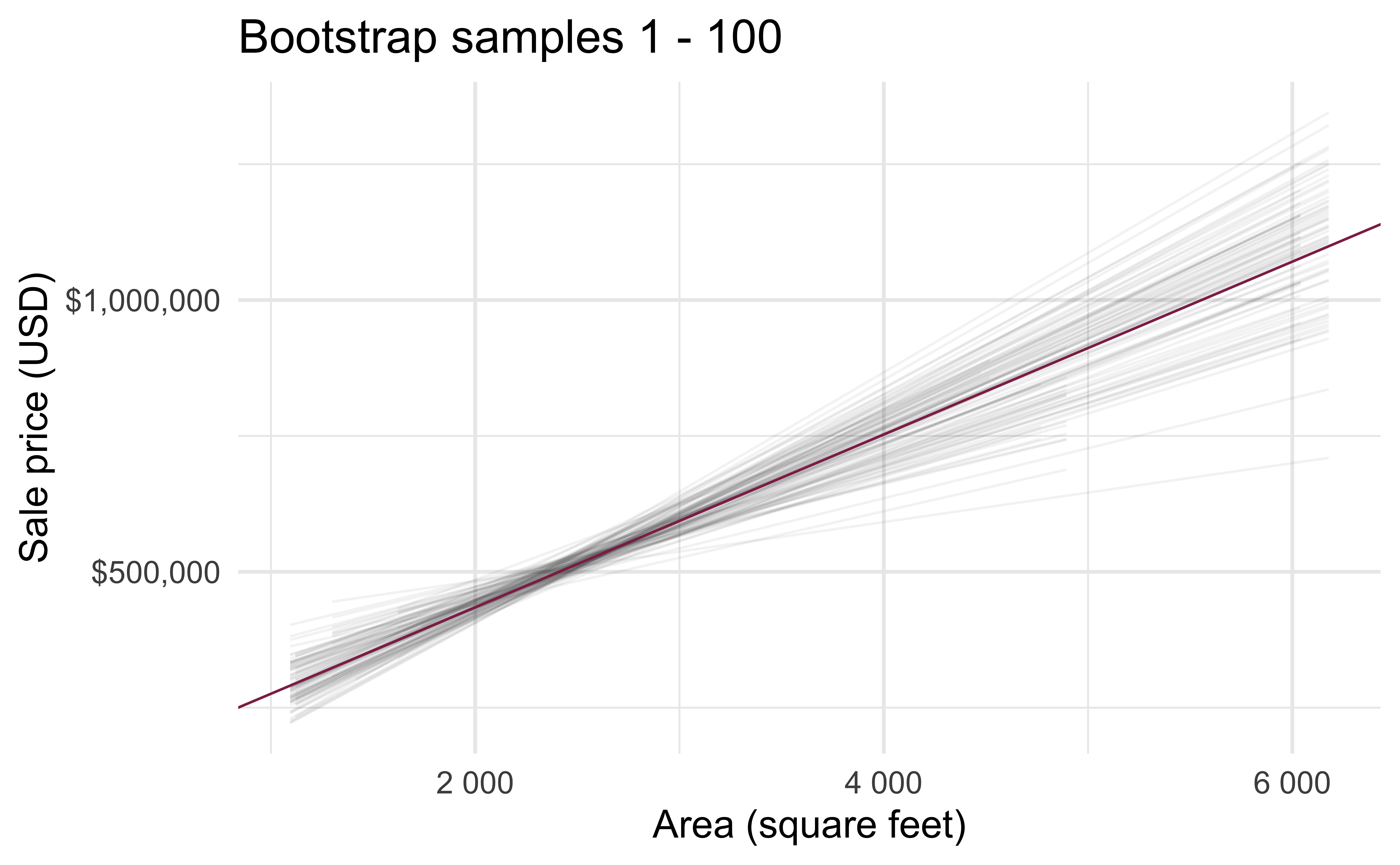
Bootstrap samples 1 - 100

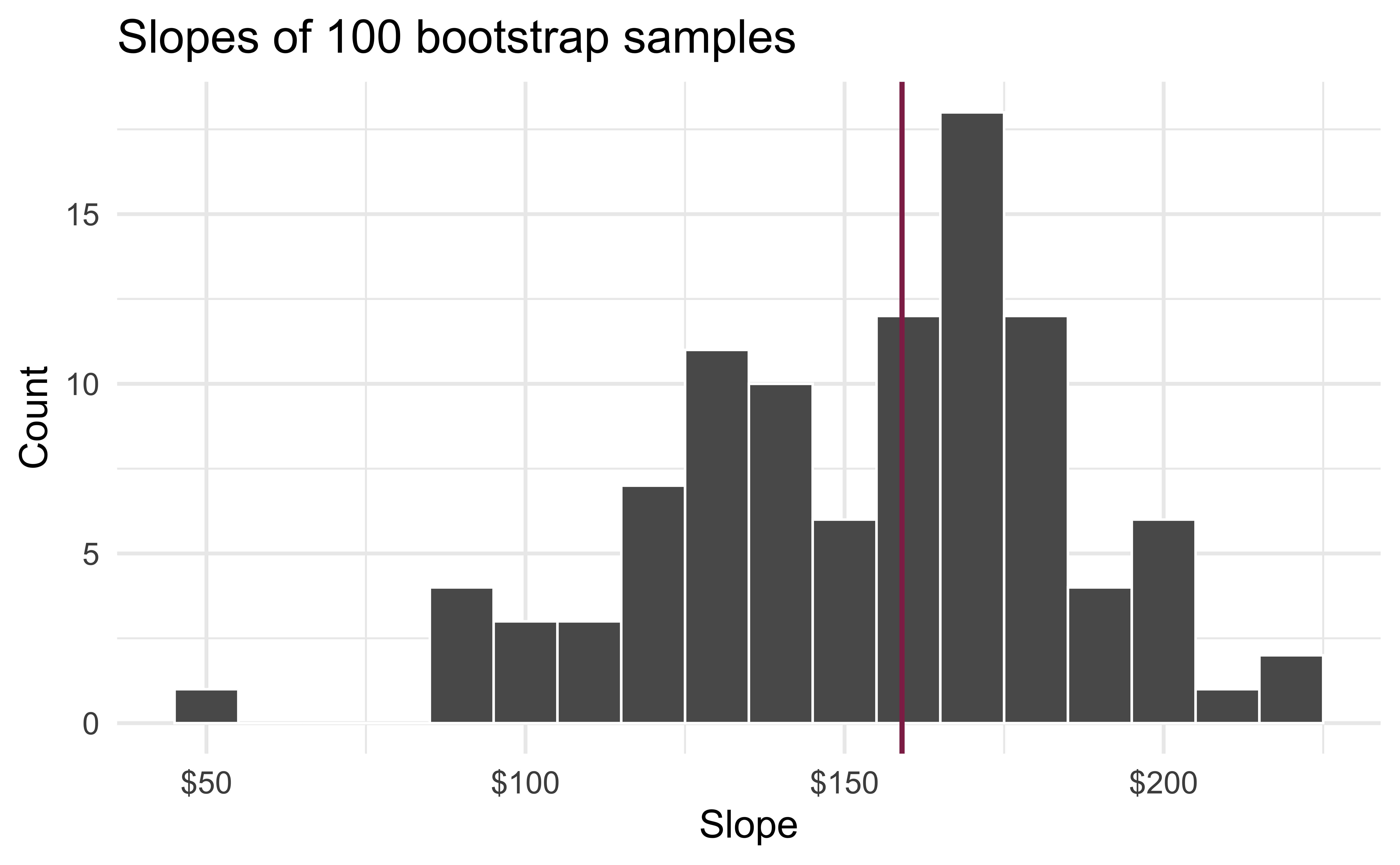
Slopes of bootstrap samples

Fill in the blank: For each additional square foot, the model predicts the sale price of Duke Forest houses to be higher, on average, by $159, give or take ___ dollars.

Slopes of bootstrap samples

Fill in the blank: For each additional square foot, the model predicts the sale price of Duke Forest houses to be higher, on average, by $159, give or take ___ dollars.

Confidence level

How confident are you that the true slope is between $0 and $250? How about $150 and $170? How about $90 and $210?

95% confidence interval

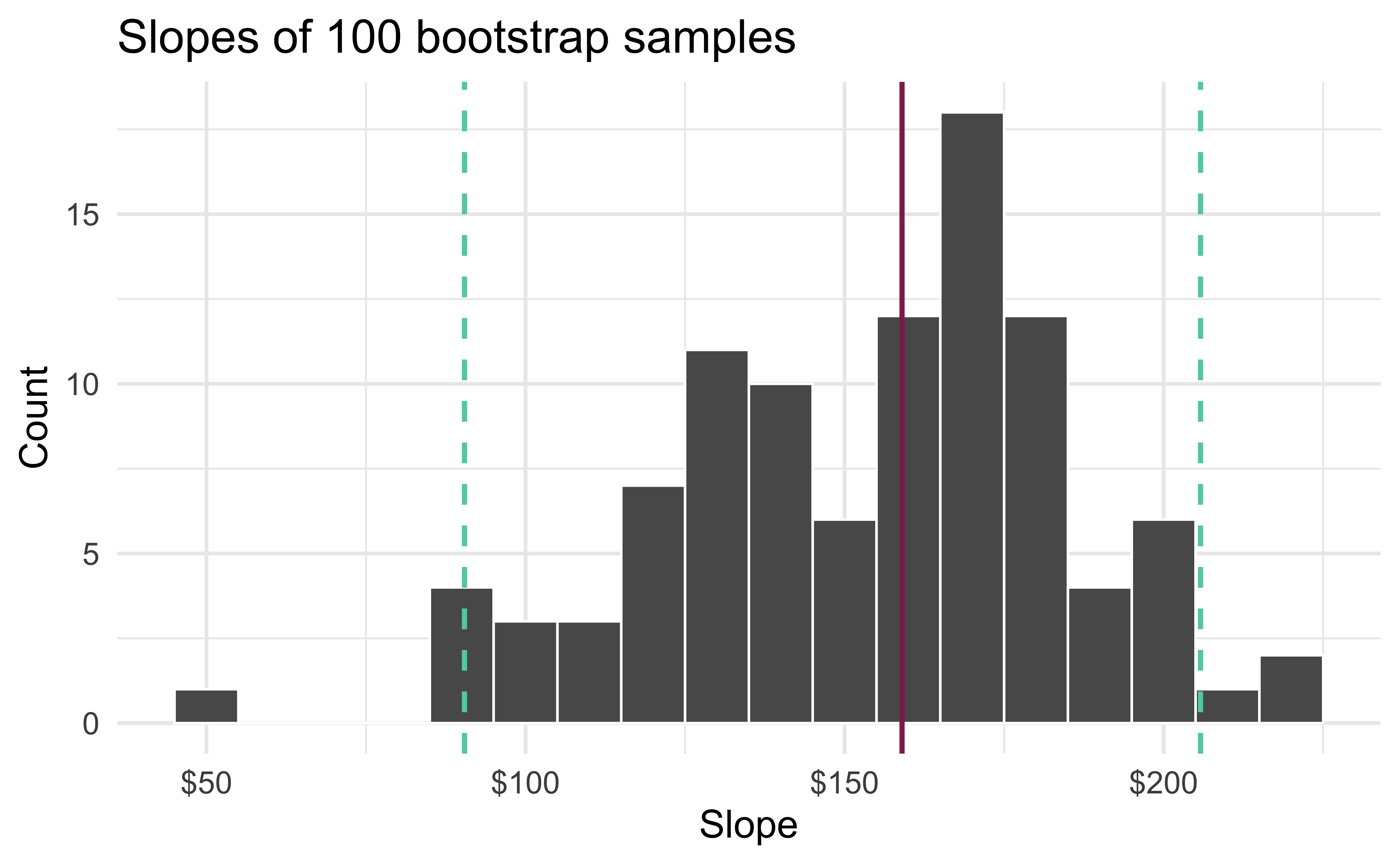
A 95% confidence interval is bounded by the middle 95% of the bootstrap distribution
We are 95% confident that For each additional square foot, the model predicts the sale price of Duke Forest houses to be higher, on average, by $90.43 to $205.77.

Computing the CI for the slope I

Calculate the observed slope:

observed_fit <- duke_forest %>%
  specify(price ~ area) %>%
  fit()

observed_fit

# A tibble: 2 × 2
  term      estimate
  <chr>        <dbl>
1 intercept  116652.
2 area          159.

Computing the CI for the slope II

Take 100 bootstrap samples and fit models to each one:

# #| code-line-numbers: "1,5,6"

set.seed(1120)

boot_fits <- duke_forest %>%
  specify(price ~ area) %>%
  generate(reps = 100, type = "bootstrap") %>%
  fit()

boot_fits

# A tibble: 200 × 3
# Groups:   replicate [100]
   replicate term      estimate
       <int> <chr>        <dbl>
 1         1 intercept   47819.
 2         1 area          191.
 3         2 intercept  144645.
 4         2 area          134.
 5         3 intercept  114008.
 6         3 area          161.
 7         4 intercept  100639.
 8         4 area          166.
 9         5 intercept  215264.
10         5 area          125.
# … with 190 more rows

Computing the CI for the slope III

Percentile method: Compute the 95% CI as the middle 95% of the bootstrap distribution:

# #| code-line-numbers: "5"

get_confidence_interval(
  boot_fits, 
  point_estimate = observed_fit, 
  level = 0.95,
  type = "percentile"
)

# A tibble: 2 × 3
  term      lower_ci upper_ci
  <chr>        <dbl>    <dbl>
1 area          92.1     223.
2 intercept -36765.   296528.

Computing the CI for the slope IV

Standard error method: Alternatively, compute the 95% CI as the point estimate $\pm$ ~2 standard deviations of the bootstrap distribution:

# #| code-line-numbers: "5"

get_confidence_interval(
  boot_fits, 
  point_estimate = observed_fit, 
  level = 0.95,
  type = "se"
)

# A tibble: 2 × 3
  term      lower_ci upper_ci
  <chr>        <dbl>    <dbl>
1 area          90.8     228.
2 intercept -56788.   290093.

Precision vs. accuracy

If we want to be very certain that we capture the population parameter, should we use a wider or a narrower interval? What drawbacks are associated with using a wider interval?

Precision vs. accuracy

How can we get best of both worlds – high precision and high accuracy?

Changing confidence level

How would you modify the following code to calculate a 90% confidence interval? How would you modify it for a 99% confidence interval?

# #| code-line-numbers: "|4"

get_confidence_interval(
  boot_fits, 
  point_estimate = observed_fit, 
  level = 0.95,
  type = "percentile"
)

# A tibble: 2 × 3
  term      lower_ci upper_ci
  <chr>        <dbl>    <dbl>
1 area          92.1     223.
2 intercept -36765.   296528.

Changing confidence level

## confidence level: 90%
get_confidence_interval(
  boot_fits, point_estimate = observed_fit, 
  level = 0.90, type = "percentile"
)

# A tibble: 2 × 3
  term      lower_ci upper_ci
  <chr>        <dbl>    <dbl>
1 area          104.     212.
2 intercept  -24380.  256730.

## confidence level: 99%
get_confidence_interval(
  boot_fits, point_estimate = observed_fit, 
  level = 0.99, type = "percentile"
)

# A tibble: 2 × 3
  term      lower_ci upper_ci
  <chr>        <dbl>    <dbl>
1 area          56.3     226.
2 intercept -61950.   370395.

Recap

Population: Complete set of observations of whatever we are studying, e.g., people, tweets, photographs, etc. (population size = $N$)
Sample: Subset of the population, ideally random and representative (sample size = $n$)
Sample statistic $\ne$ population parameter, but if the sample is good, it can be a good estimate
Statistical inference: Discipline that concerns itself with the development of procedures, methods, and theorems that allow us to extract meaning and information from data that has been generated by stochastic (random) process
We report the estimate with a confidence interval, and the width of this interval depends on the variability of sample statistics from different samples from the population
Since we can’t continue sampling from the population, we bootstrap from the one sample we have to estimate sampling variability

Sampling is natural

When you taste a spoonful of soup and decide the spoonful you tasted isn’t salty enough, that’s exploratory analysis
If you generalize and conclude that your entire soup needs salt, that’s an inference
For your inference to be valid, the spoonful you tasted (the sample) needs to be representative of the entire pot (the population)

Hypothesis test for the slope

Statistical significance

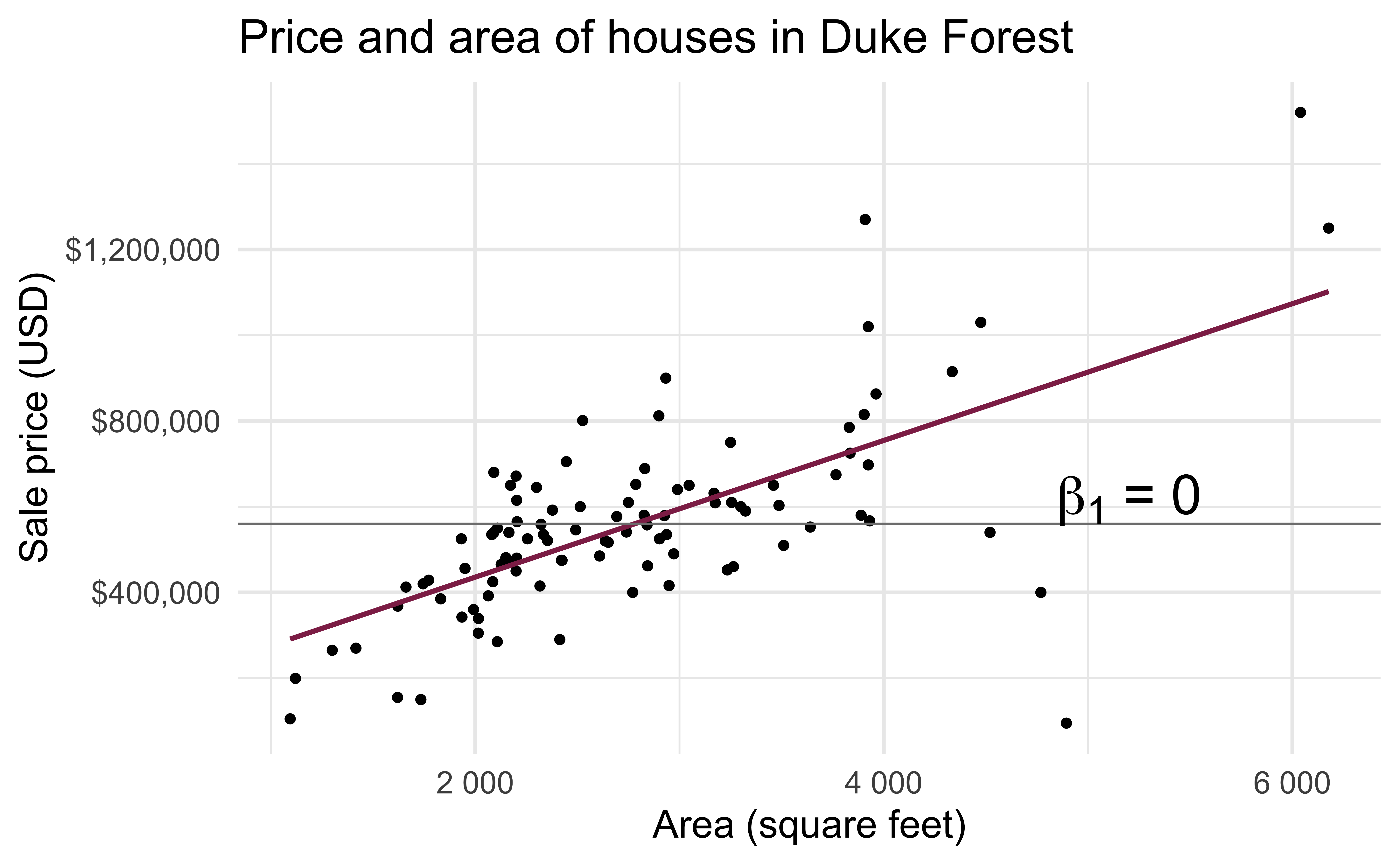
Do the data provide sufficient evidence that $\beta_1$ (the true slope for the population) is different from 0?

Hypotheses

We want to answer the question “Do the data provide sufficient evidence that $\beta_1$ (the true slope for the population) is different from 0?”
Null hypothesis - $H_0: \beta_1 = 0$, there is no linear relationship between area and price
Alternative hypothesis - $H_A: \beta_1 \ne 0$, there is a linear relationship between area and price

Hypothesis testing as a court trial

Null hypothesis, $H_0$: Defendant is innocent
Alternative hypothesis, $H_A$: Defendant is guilty
Present the evidence: Collect data
Judge the evidence: “Could these data plausibly have happened by chance if the null hypothesis were true?”
- Yes: Fail to reject $H_0$
- No: Reject $H_0$

Hypothesis testing framework

Start with a null hypothesis, $H_0$ that represents the status quo
Set an alternative hypothesis, $H_A$ that represents the research question, i.e. what we’re testing for
Conduct a hypothesis test under the assumption that the null hypothesis is true and calculate a p-value (probability of observed or more extreme outcome given that the null hypothesis is true)
- if the test results suggest that the data do not provide convincing evidence for the alternative hypothesis, stick with the null hypothesis
- if they do, then reject the null hypothesis in favor of the alternative