Data Wrangling
STA 210 - Summer 2022
Data Cleaning using tidyverse
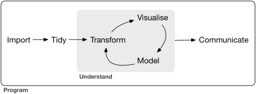
Raw data to understanding, insight, and knowledge
Workflow for real-world data analysis
Packages in Tidyverse
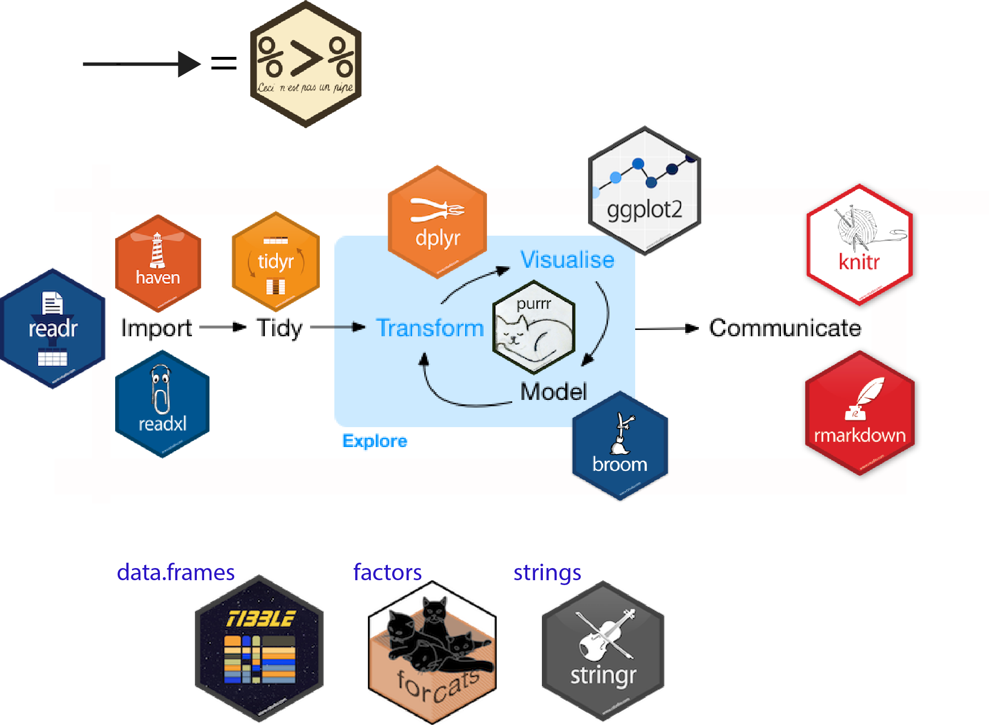
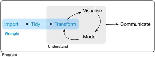
Focus on data wrangling
Data import (
readr,tibble)Tidy data (
tidyr)Wrangle (
dplyr,stringr,lubridate,janitor)
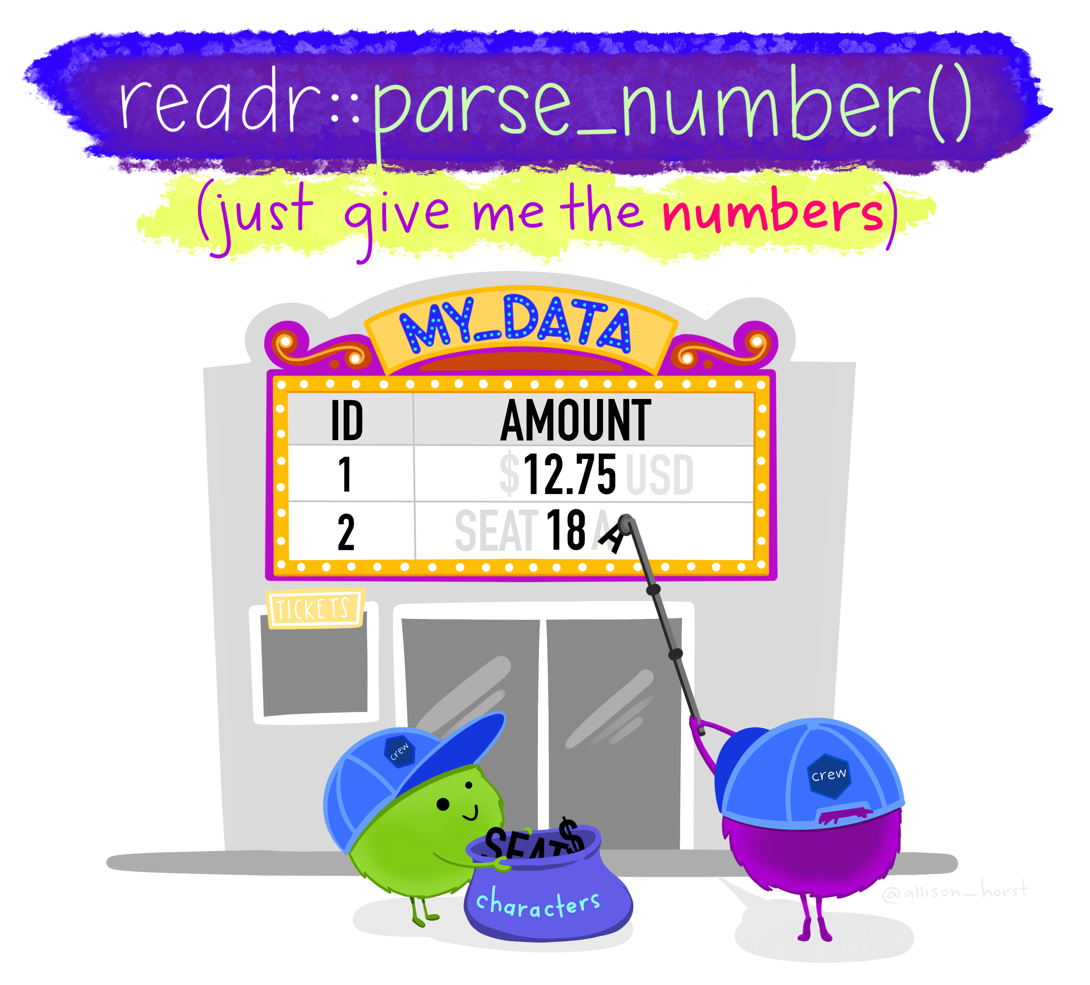
Extract the certain type of data
readr::parse_*: parse the characters/numbers only
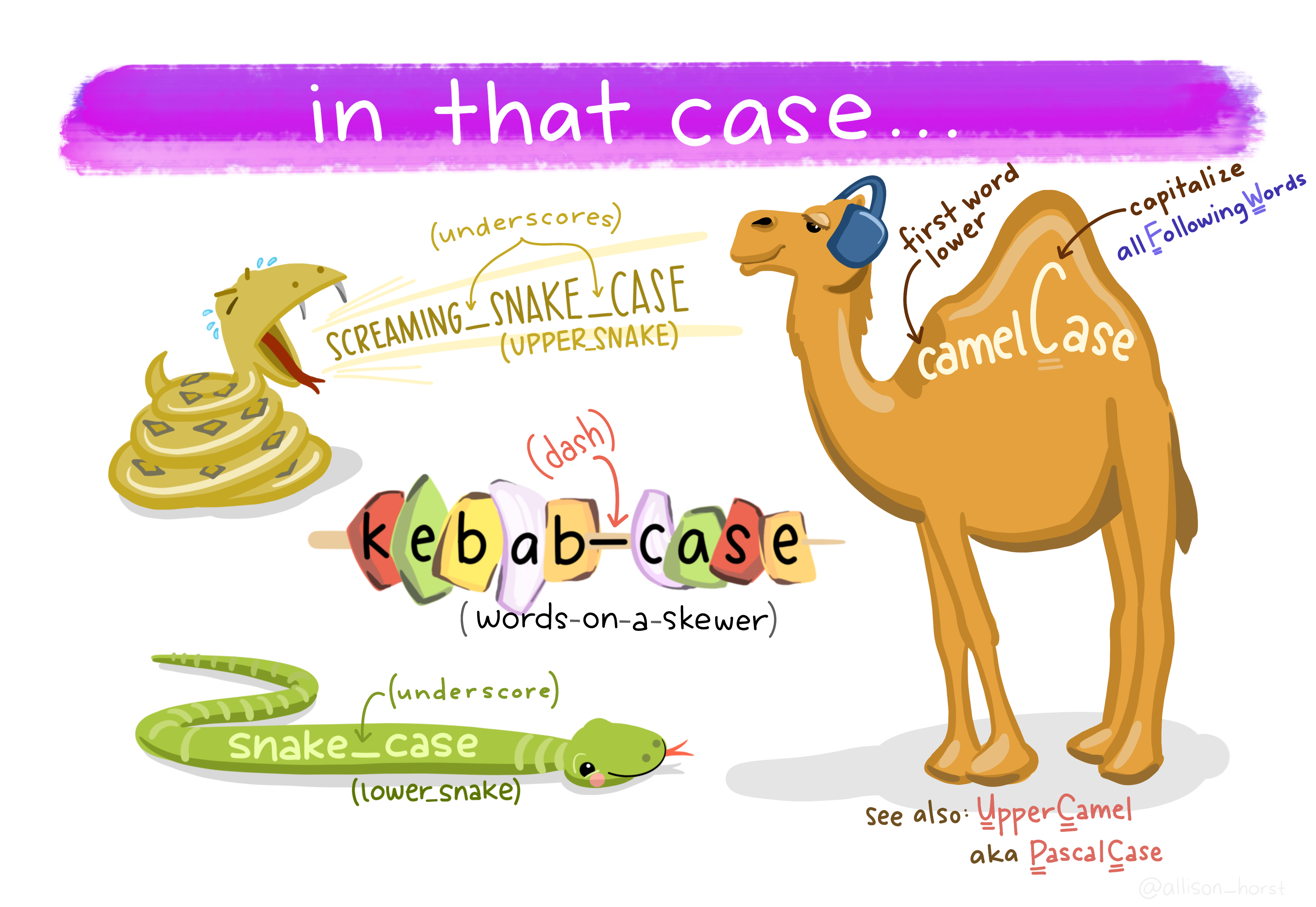
janitor package can help with cleaning names
clean_names,remove_empty_cols,remove_empty_rows
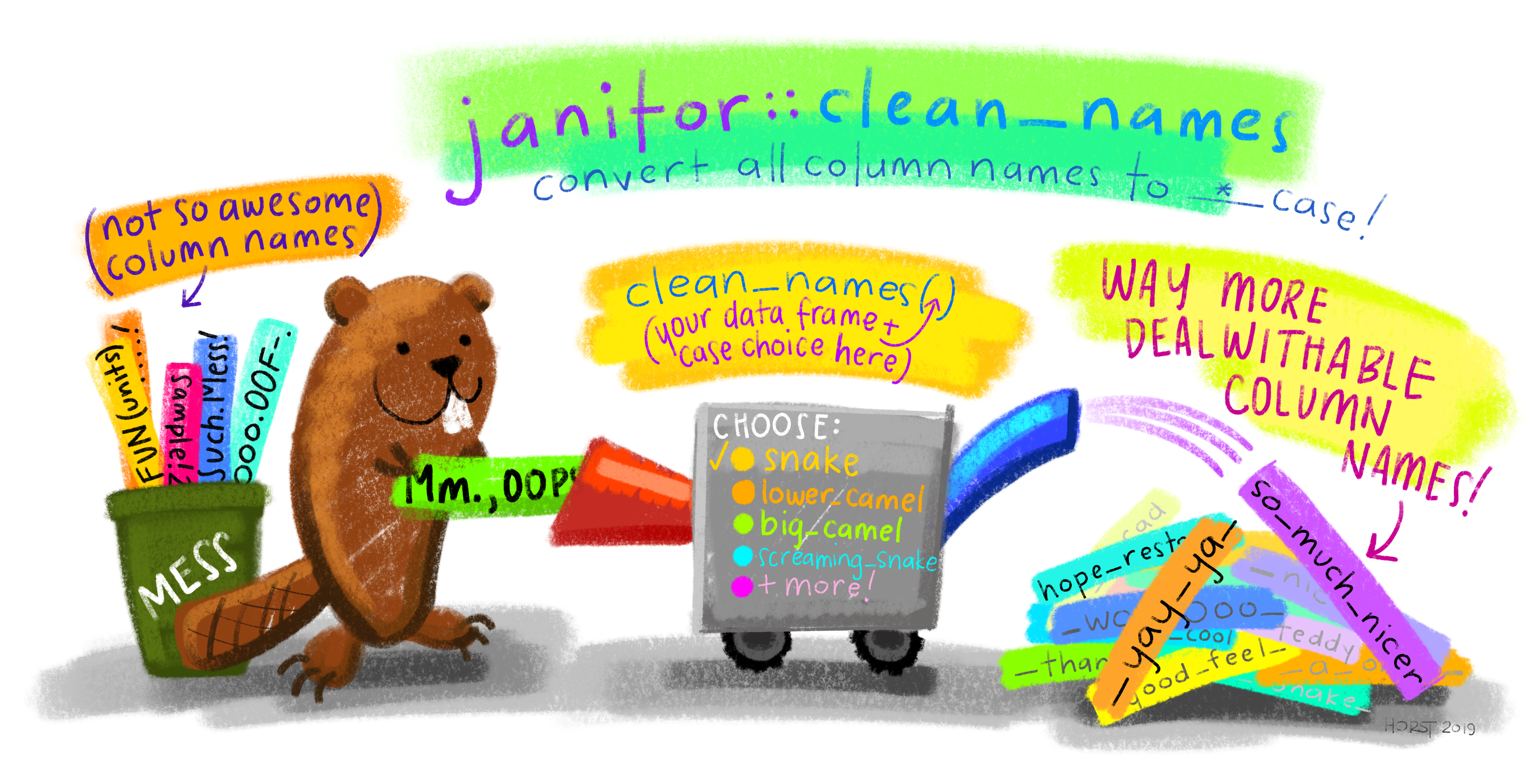
janitor package
clean_names,remove_empty_cols,remove_empty_rows
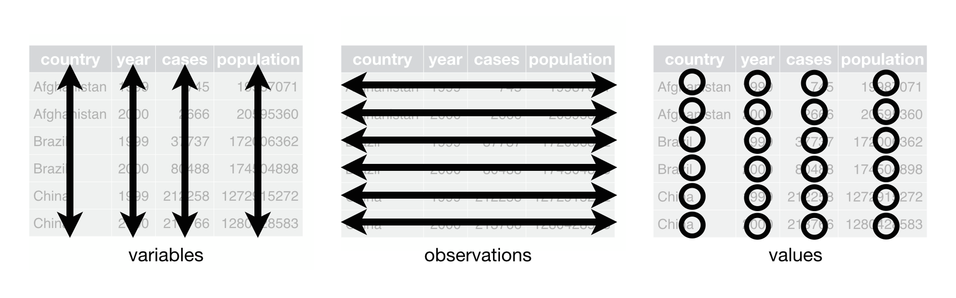
Tidy data
Tidy data
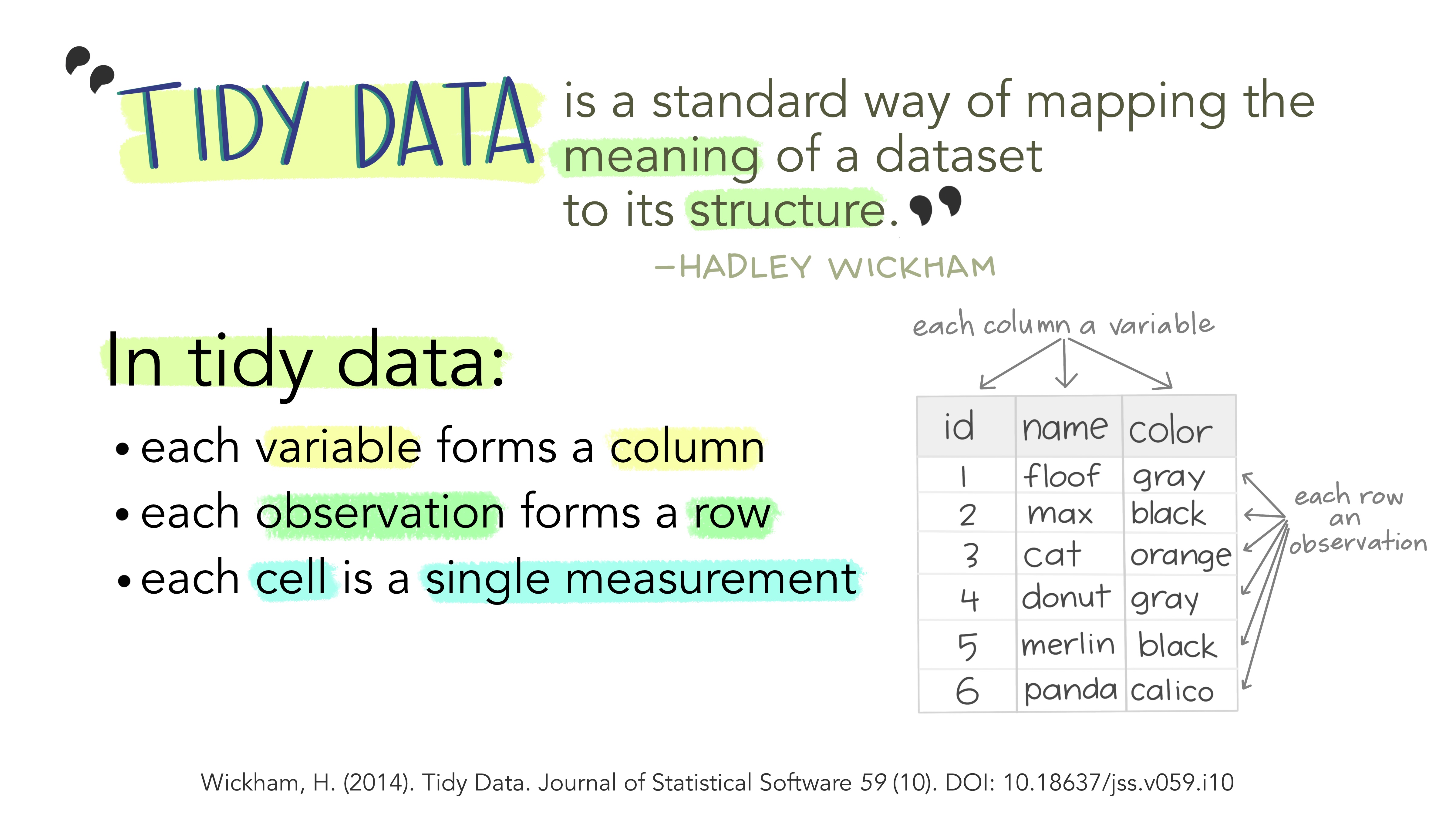
Tidy data
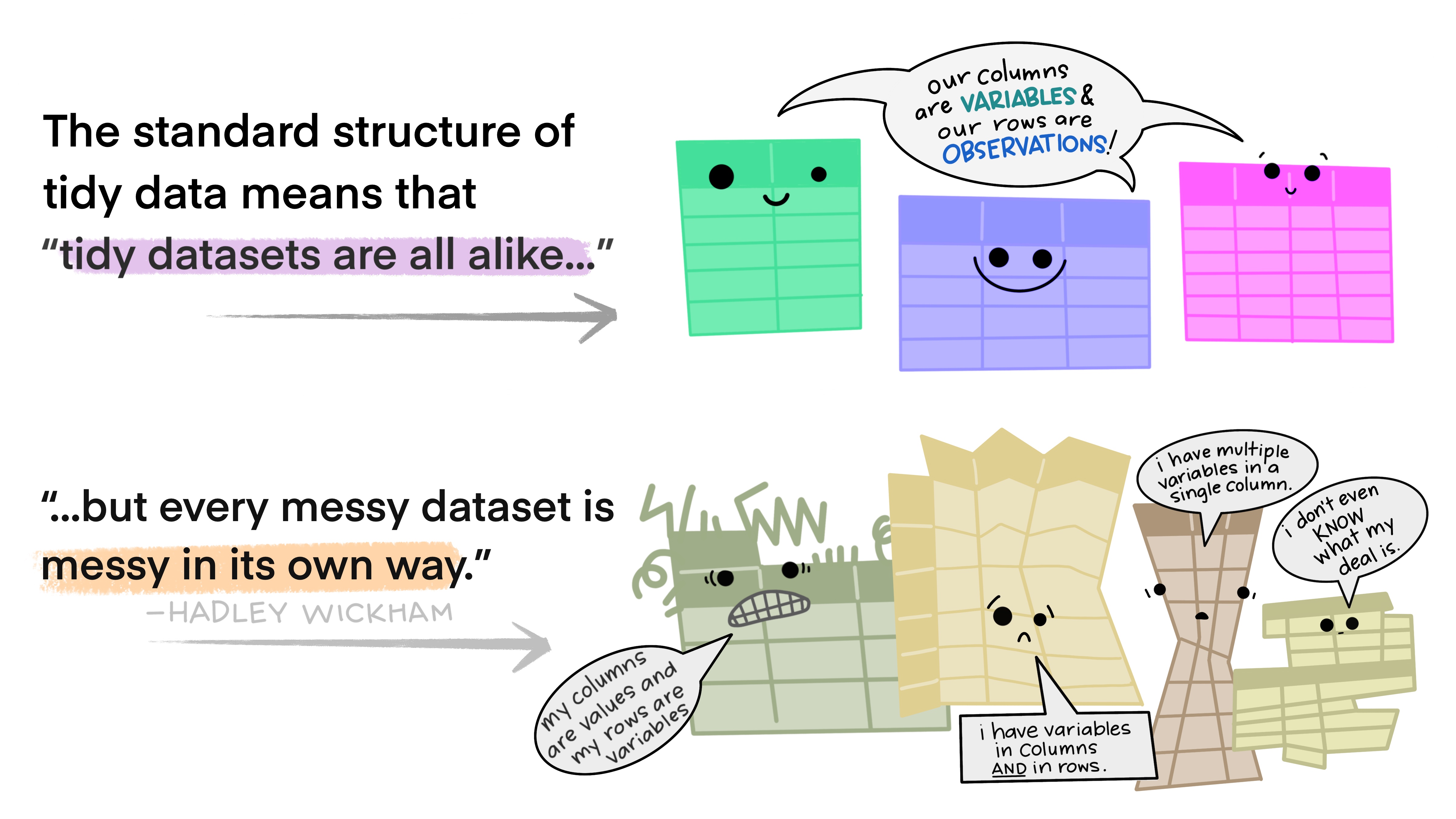
Tidy data
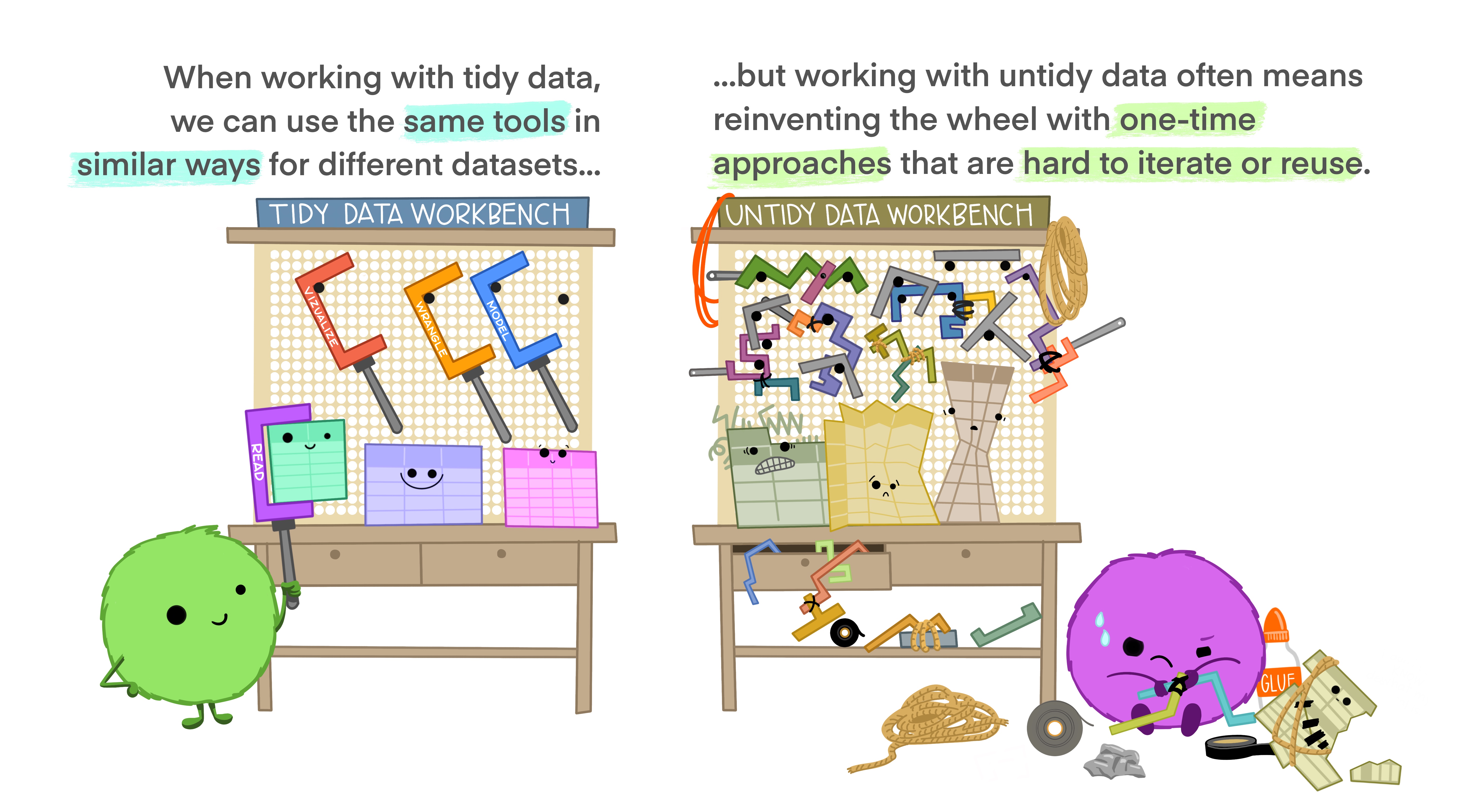
Tidy data

Tidy data
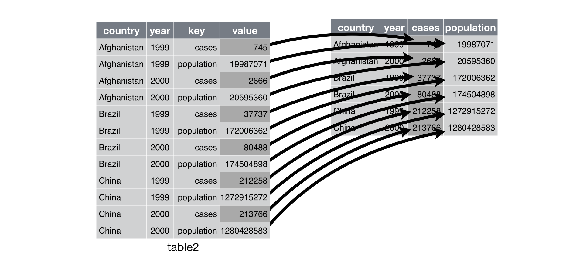
pivot_longer function in tidyr pkg
pivot_longer: from wide to long
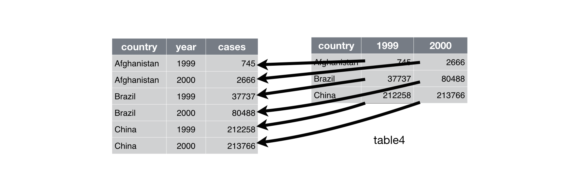
pivot_wider function in tidyr pkg
pivot_wider: from long to wide
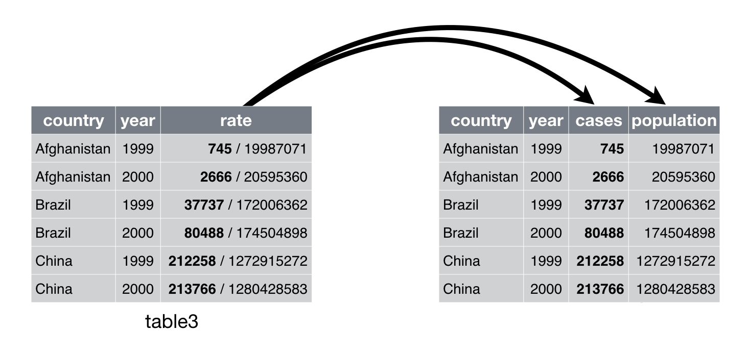
separate function in tidyr pkg
separate: from 1 column to 2+ column- can
sepbased on digits or characters.
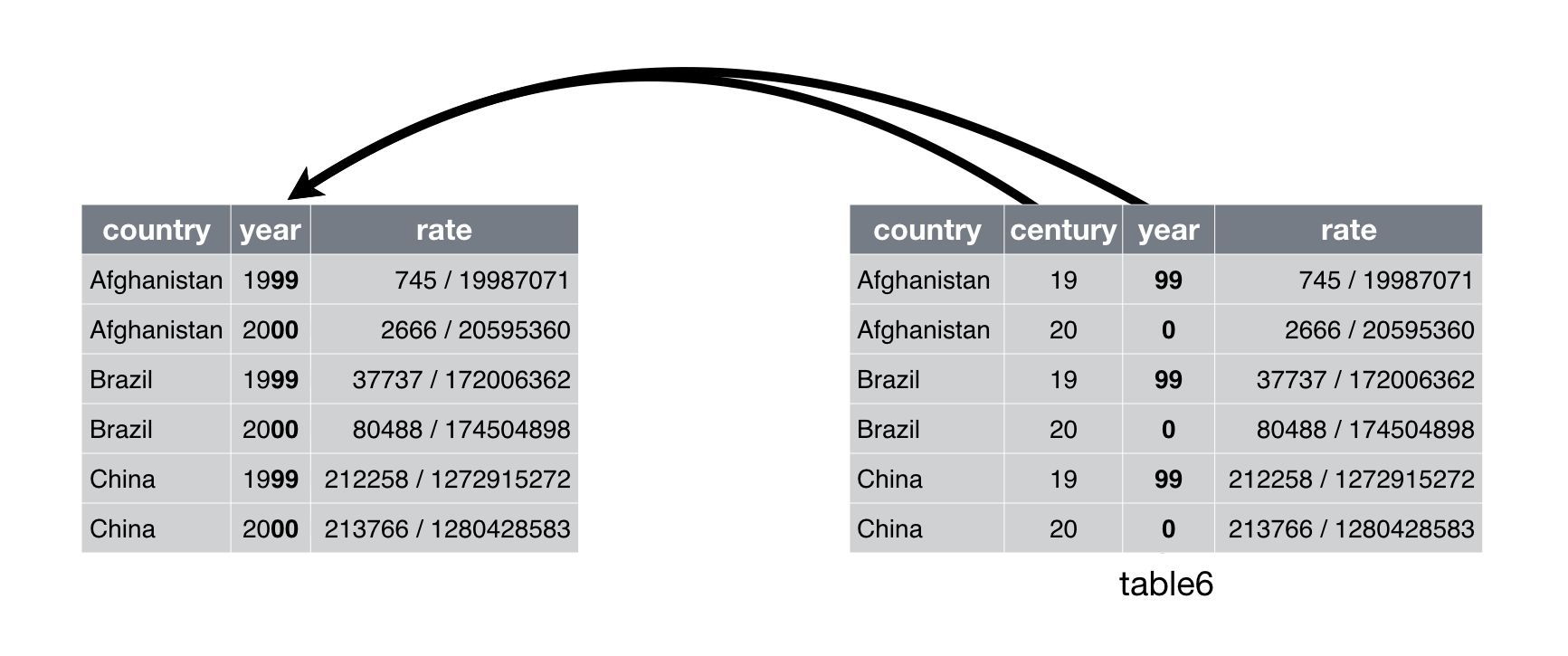
unite function in tidyr pkg
unite: from 2+ column to 1 column
Packages in Tidyverse
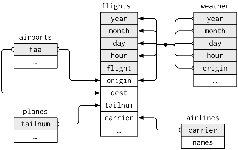
Relational datasets in nycflights13
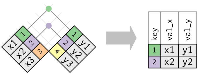
inner_join
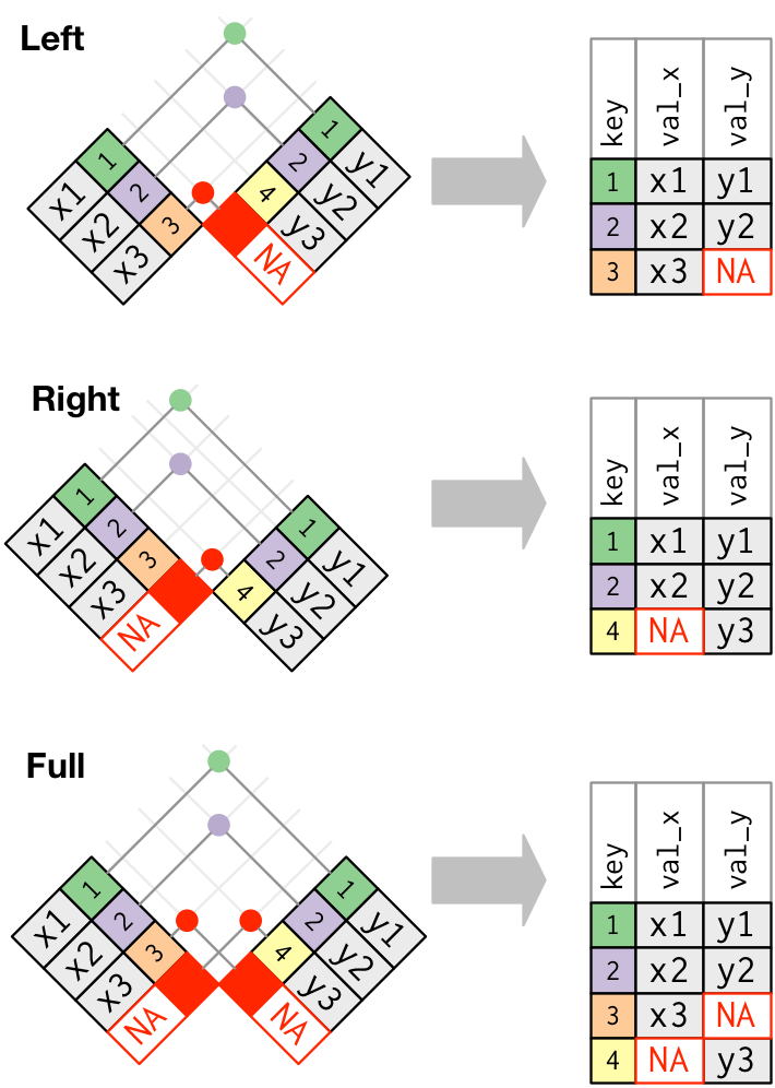
*_join
left_join, right_join, full_join
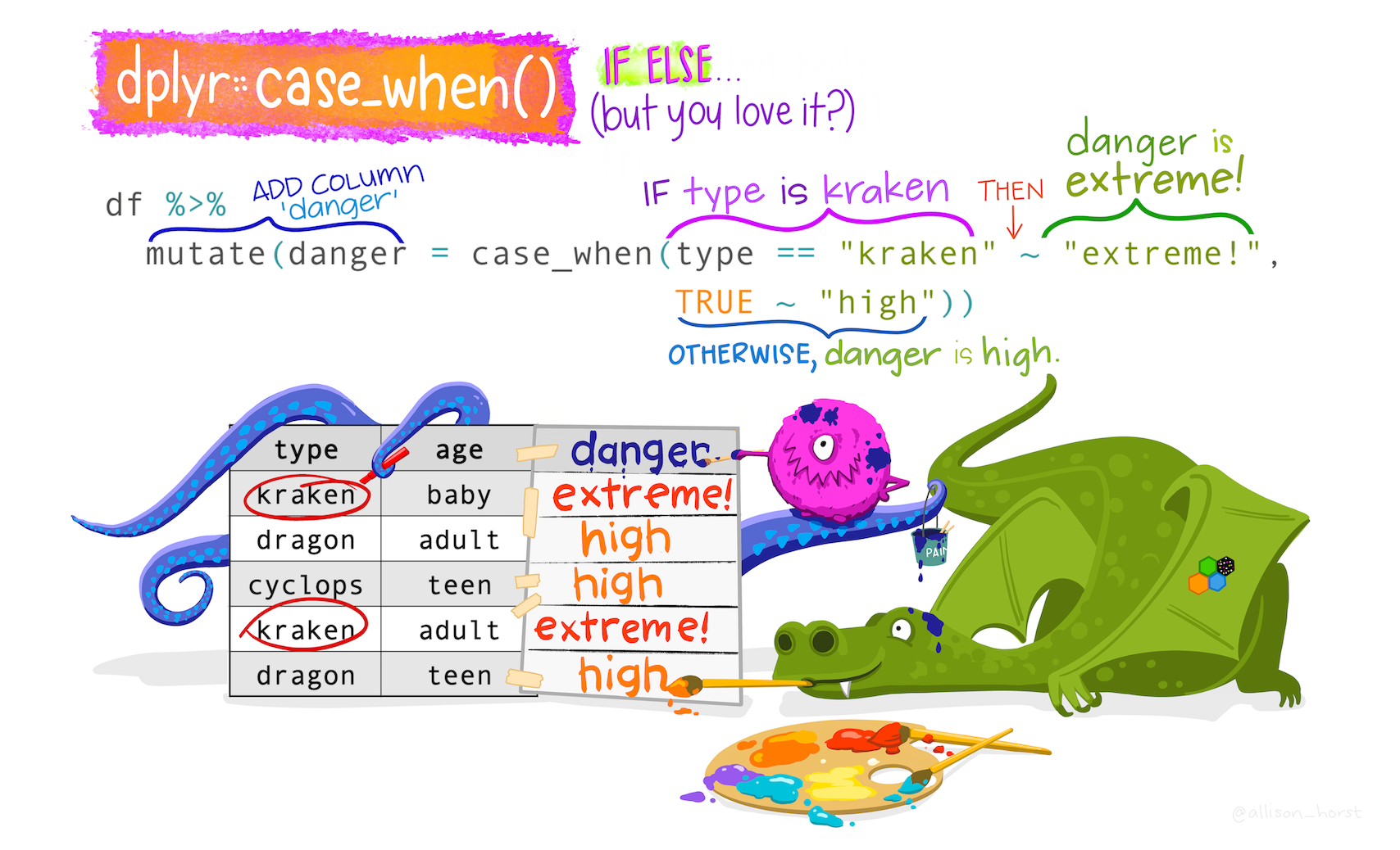
case_when
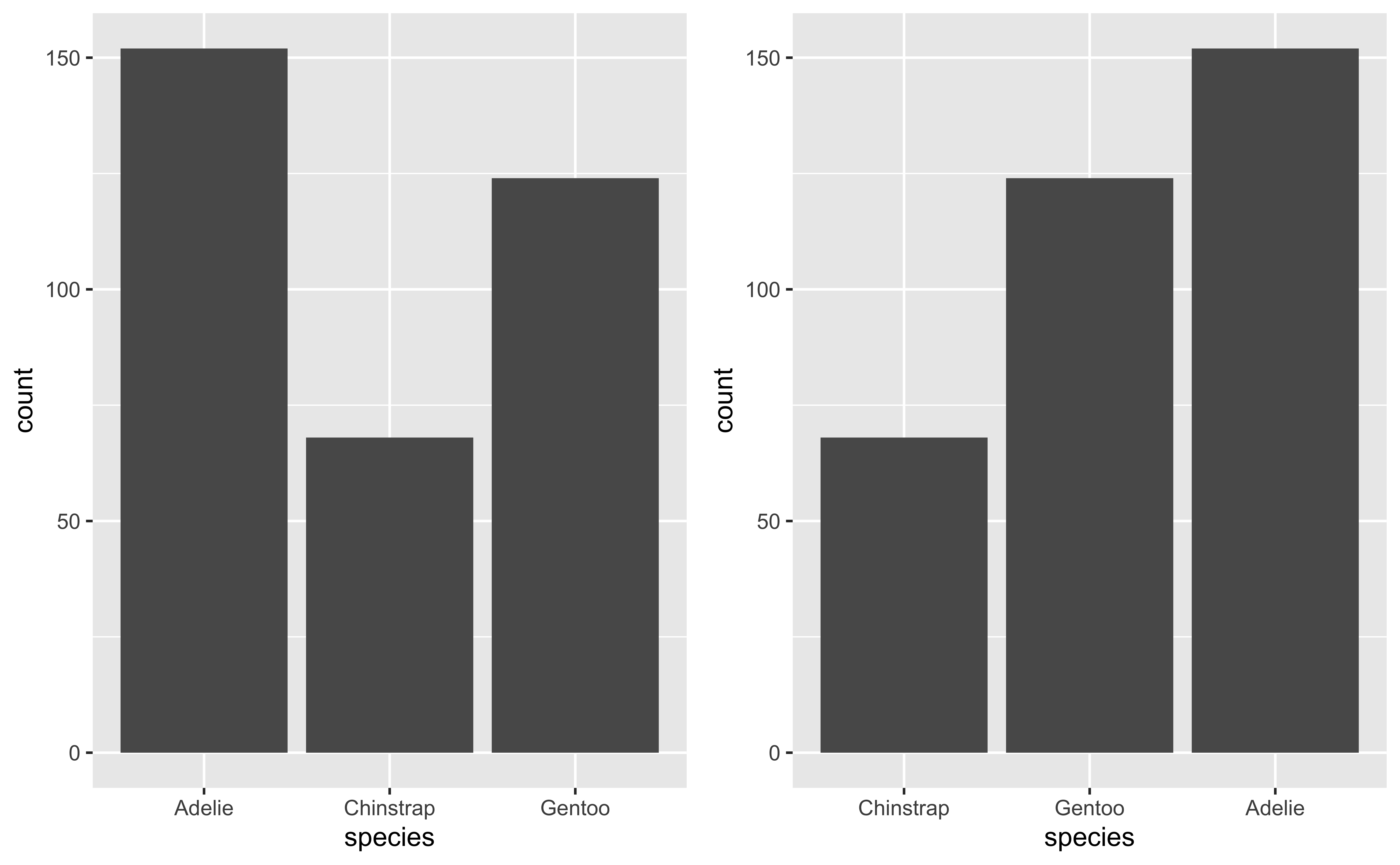
fct_infreq and fct_rev
Examples for fct_reorder
library(cowplot)
peng_summary=penguins %>%
  group_by(species)%>%
  summarise(
    bill_length_mean=mean(bill_length_mm, na.rm=T),
    bill_depth_mean=mean(bill_depth_mm, na.rm=T))
p1=ggplot(peng_summary,aes(bill_length_mean,species)) +
  geom_point()
p2=ggplot(peng_summary,aes(bill_length_mean,fct_reorder(species,bill_length_mean))) + geom_point()
plot_grid(p1,p2)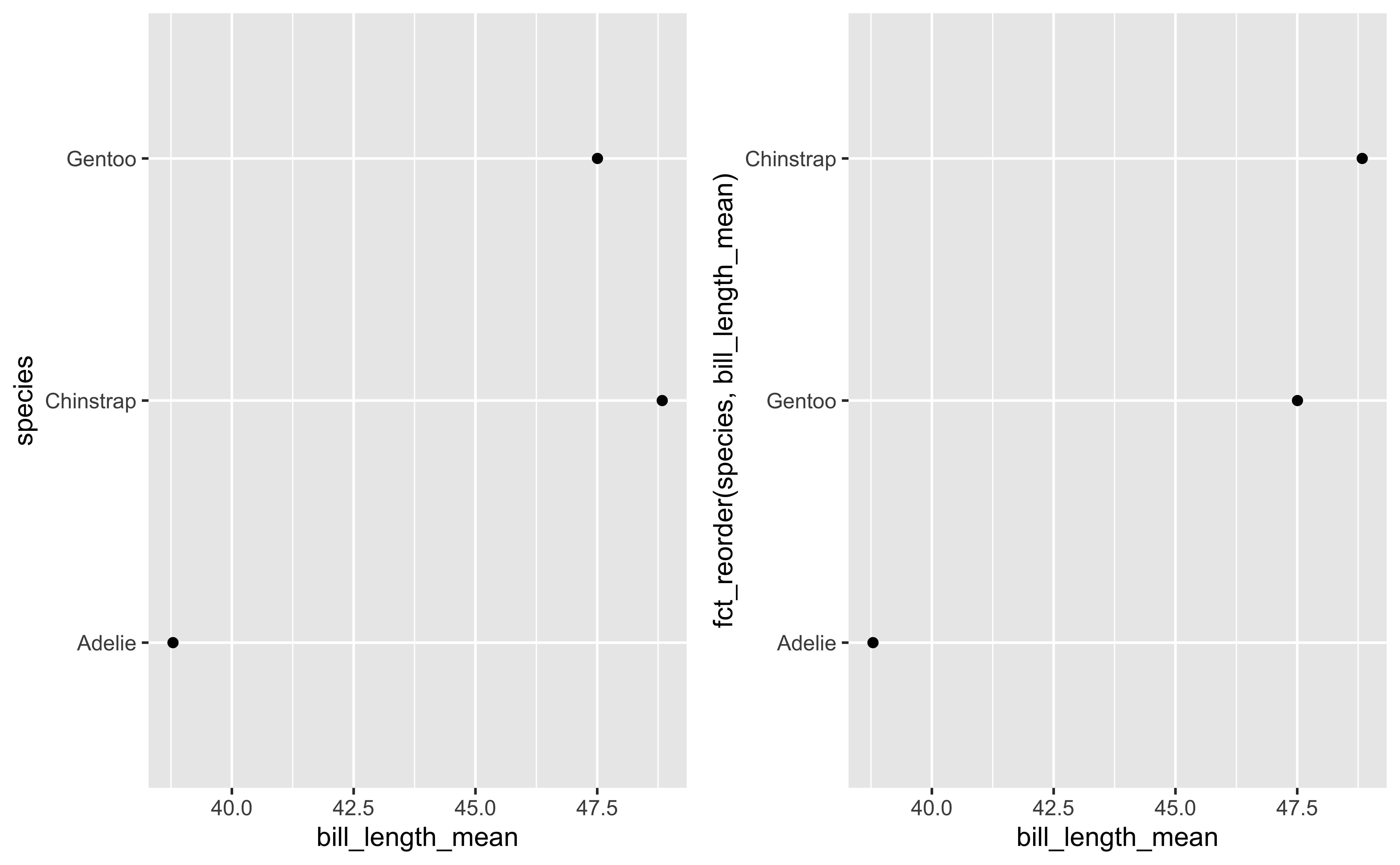
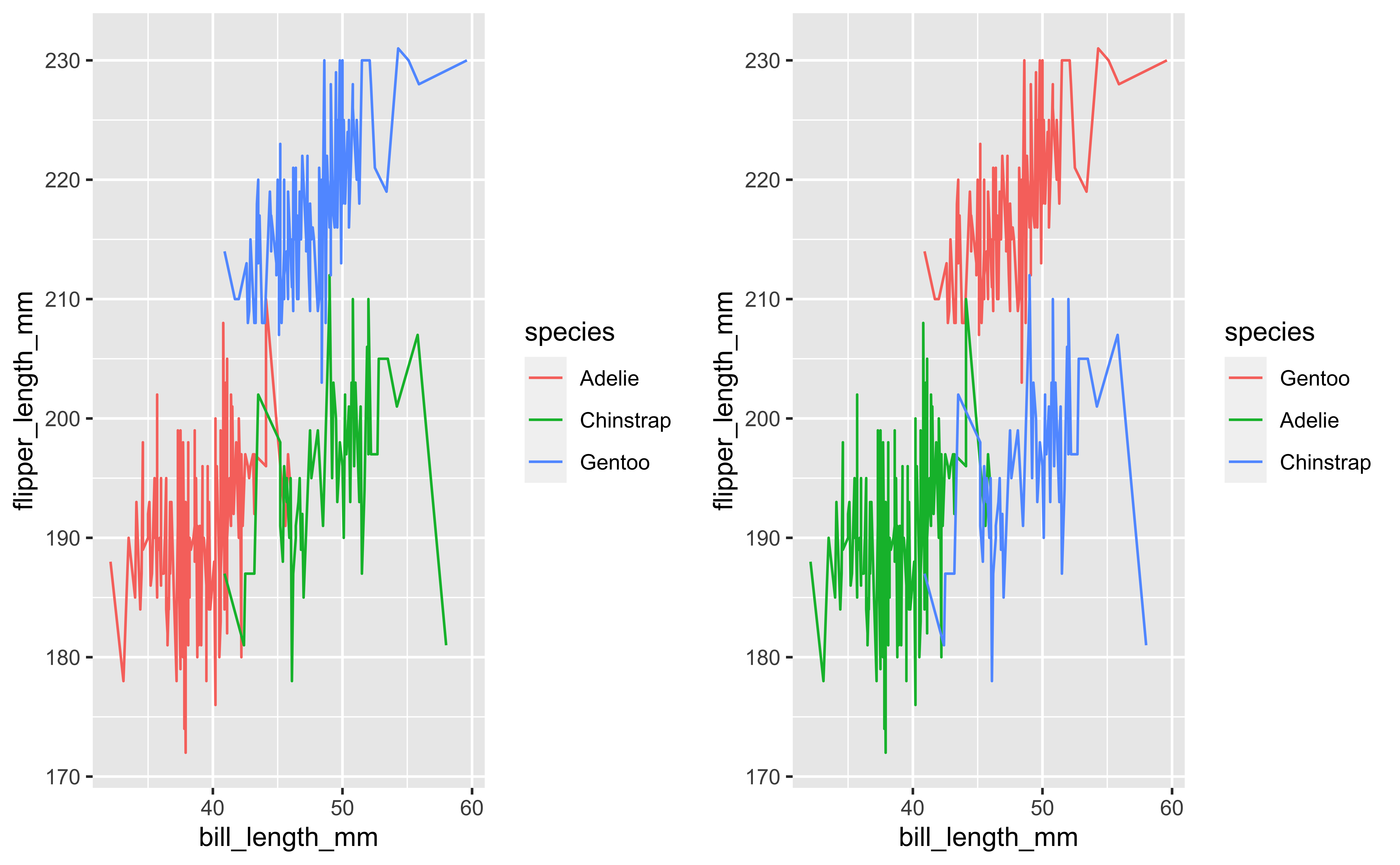
Examples for fct_reorder2
- Reorder the factor by the y values associated with the largest x values
- Easier to read: colours line up with the legend
Reference
- Allison Horst’s Posts
- Julie Scholler’s Slides
- R for Data Science
- Gina Reynolds’s Slides
- Sharla Gelfand’s Slides
- David’s Blog