Simple Linear Regression

STA 210 - Summer 2022

Yunran Chen

Welcome

Announcements

• If you’re just joining the class, welcome! Go to the course website and review content you’ve missed, read the syllabus, and complete the Getting to know you survey.
• Lab 1 is due Friday, at 11:59pm, on Gradescope.

Review on Lab 1

• Get used to R and R studio

• Get used to use R with Git : clone, commit, pull, push

• Learn the components of drawing a plot

  • data
  • mapping (x,y,color,alpha)
  • geometry (histogram, point, density)
  • lab (label for x,y-axises, title, etc.)
  • Check cheatsheet

Review on Lab 1

• Questions:

  • Choice of binwidth for histogram: Pick the one and reveal the main trend. Too small: too noisy; Too large: ignore trend
  • Density Plot (Smooth version of histogram. eg. Normal Distribution)

Outline

• Use simple linear regression to describe the relationship between a quantitative predictor and quantitative outcome variable

• Estimate the slope and intercept of the regression line using the least squares method

• Interpret the slope and intercept of the regression line

Computational setup

# load packages
library(tidyverse)       # for data wrangling
library(tidymodels)      # for modeling
library(fivethirtyeight) # for the fandango dataset

# set default theme and larger font size for ggplot2
ggplot2::theme_set(ggplot2::theme_minimal(base_size = 16))

# set default figure parameters for knitr
knitr::opts_chunk$set(
  fig.width = 8,
  fig.asp = 0.618,
  fig.retina = 3,
  dpi = 300,
  out.width = "80%"
)

Data

Movie ratings

• Data behind the FiveThirtyEight story Be Suspicious Of Online Movie Ratings, Especially Fandango’s
• In the fivethirtyeight package: fandango
• Contains every film that has at least 30 fan reviews on Fandango, an IMDb score, Rotten Tomatoes critic and user ratings, and Metacritic critic and user scores

Data prep

• Rename Rotten Tomatoes columns as critics and audience
• Rename the dataset as movie_scores

movie_scores <- fandango %>%
  rename(
    critics = rottentomatoes, 
    audience = rottentomatoes_user
  )

Data overview

glimpse(movie_scores)

Rows: 146
Columns: 23
$ film                       <chr> "Avengers: Age of Ultron", "Cinderella", "A…
$ year                       <dbl> 2015, 2015, 2015, 2015, 2015, 2015, 2015, 2…
$ critics                    <int> 74, 85, 80, 18, 14, 63, 42, 86, 99, 89, 84,…
$ audience                   <int> 86, 80, 90, 84, 28, 62, 53, 64, 82, 87, 77,…
$ metacritic                 <int> 66, 67, 64, 22, 29, 50, 53, 81, 81, 80, 71,…
$ metacritic_user            <dbl> 7.1, 7.5, 8.1, 4.7, 3.4, 6.8, 7.6, 6.8, 8.8…
$ imdb                       <dbl> 7.8, 7.1, 7.8, 5.4, 5.1, 7.2, 6.9, 6.5, 7.4…
$ fandango_stars             <dbl> 5.0, 5.0, 5.0, 5.0, 3.5, 4.5, 4.0, 4.0, 4.5…
$ fandango_ratingvalue       <dbl> 4.5, 4.5, 4.5, 4.5, 3.0, 4.0, 3.5, 3.5, 4.0…
$ rt_norm                    <dbl> 3.70, 4.25, 4.00, 0.90, 0.70, 3.15, 2.10, 4…
$ rt_user_norm               <dbl> 4.30, 4.00, 4.50, 4.20, 1.40, 3.10, 2.65, 3…
$ metacritic_norm            <dbl> 3.30, 3.35, 3.20, 1.10, 1.45, 2.50, 2.65, 4…
$ metacritic_user_nom        <dbl> 3.55, 3.75, 4.05, 2.35, 1.70, 3.40, 3.80, 3…
$ imdb_norm                  <dbl> 3.90, 3.55, 3.90, 2.70, 2.55, 3.60, 3.45, 3…
$ rt_norm_round              <dbl> 3.5, 4.5, 4.0, 1.0, 0.5, 3.0, 2.0, 4.5, 5.0…
$ rt_user_norm_round         <dbl> 4.5, 4.0, 4.5, 4.0, 1.5, 3.0, 2.5, 3.0, 4.0…
$ metacritic_norm_round      <dbl> 3.5, 3.5, 3.0, 1.0, 1.5, 2.5, 2.5, 4.0, 4.0…
$ metacritic_user_norm_round <dbl> 3.5, 4.0, 4.0, 2.5, 1.5, 3.5, 4.0, 3.5, 4.5…
$ imdb_norm_round            <dbl> 4.0, 3.5, 4.0, 2.5, 2.5, 3.5, 3.5, 3.5, 3.5…
$ metacritic_user_vote_count <int> 1330, 249, 627, 31, 88, 34, 17, 124, 62, 54…
$ imdb_user_vote_count       <int> 271107, 65709, 103660, 3136, 19560, 39373, …
$ fandango_votes             <int> 14846, 12640, 12055, 1793, 1021, 397, 252, …
$ fandango_difference        <dbl> 0.5, 0.5, 0.5, 0.5, 0.5, 0.5, 0.5, 0.5, 0.5…

Data visualization

Regression model

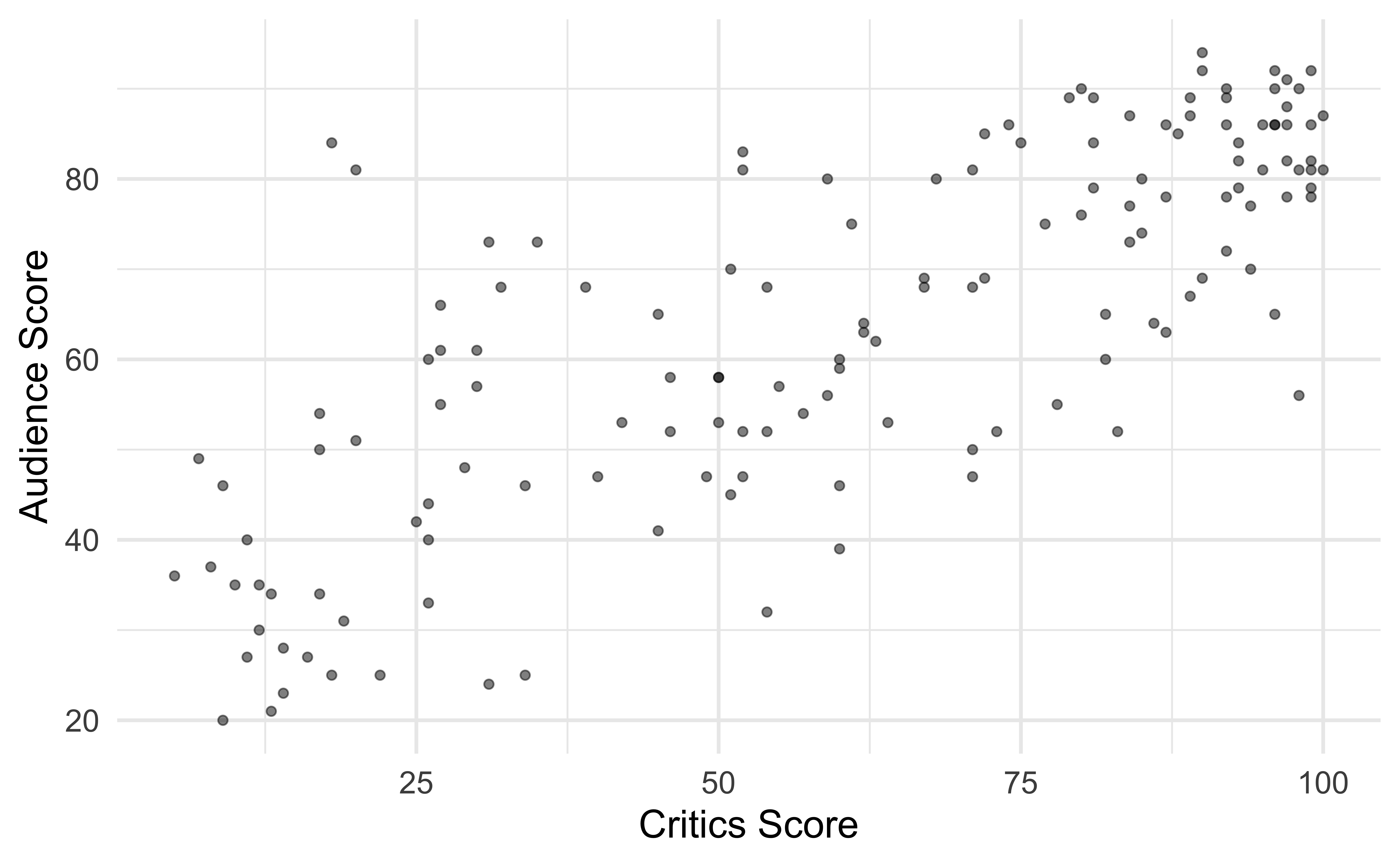
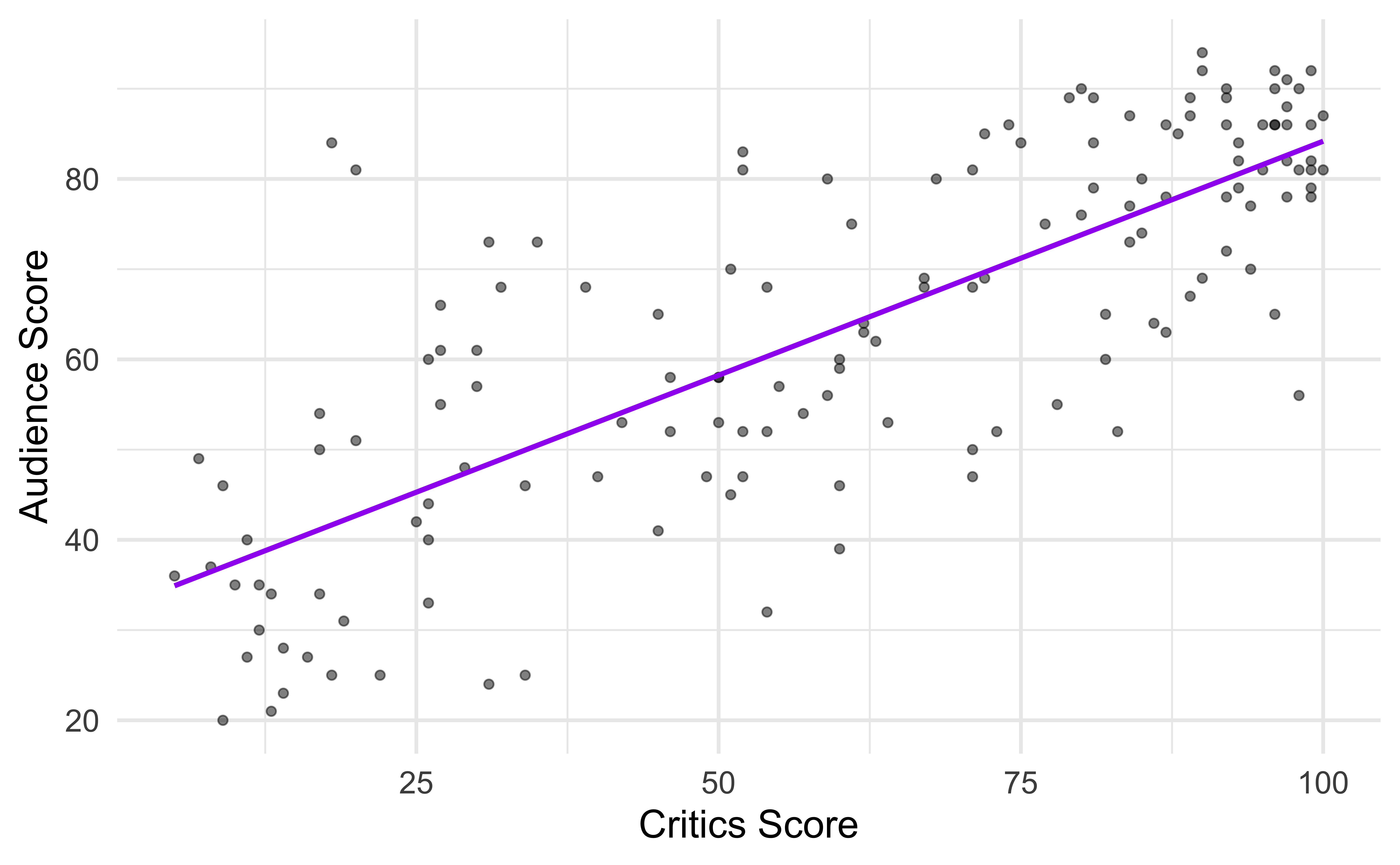
Fit a line

… to describe the relationship between the critics and audience score

Terminology

• Outcome, Y: variable describing the outcome of interest
• Predictor, X: variable used to help understand the variability in the outcome

Regression model

A regression model is a function that describes the relationship between the outcome, \(Y\), and the predictor, \(X\).

\[\begin{aligned} Y &= \color{black}{\textbf{Model}} + \text{Error} \\[8pt] &= \color{black}{\mathbf{f(X)}} + \epsilon \\[8pt] &= \color{black}{\boldsymbol{\mu_{Y|X}}} + \epsilon \end{aligned}\]

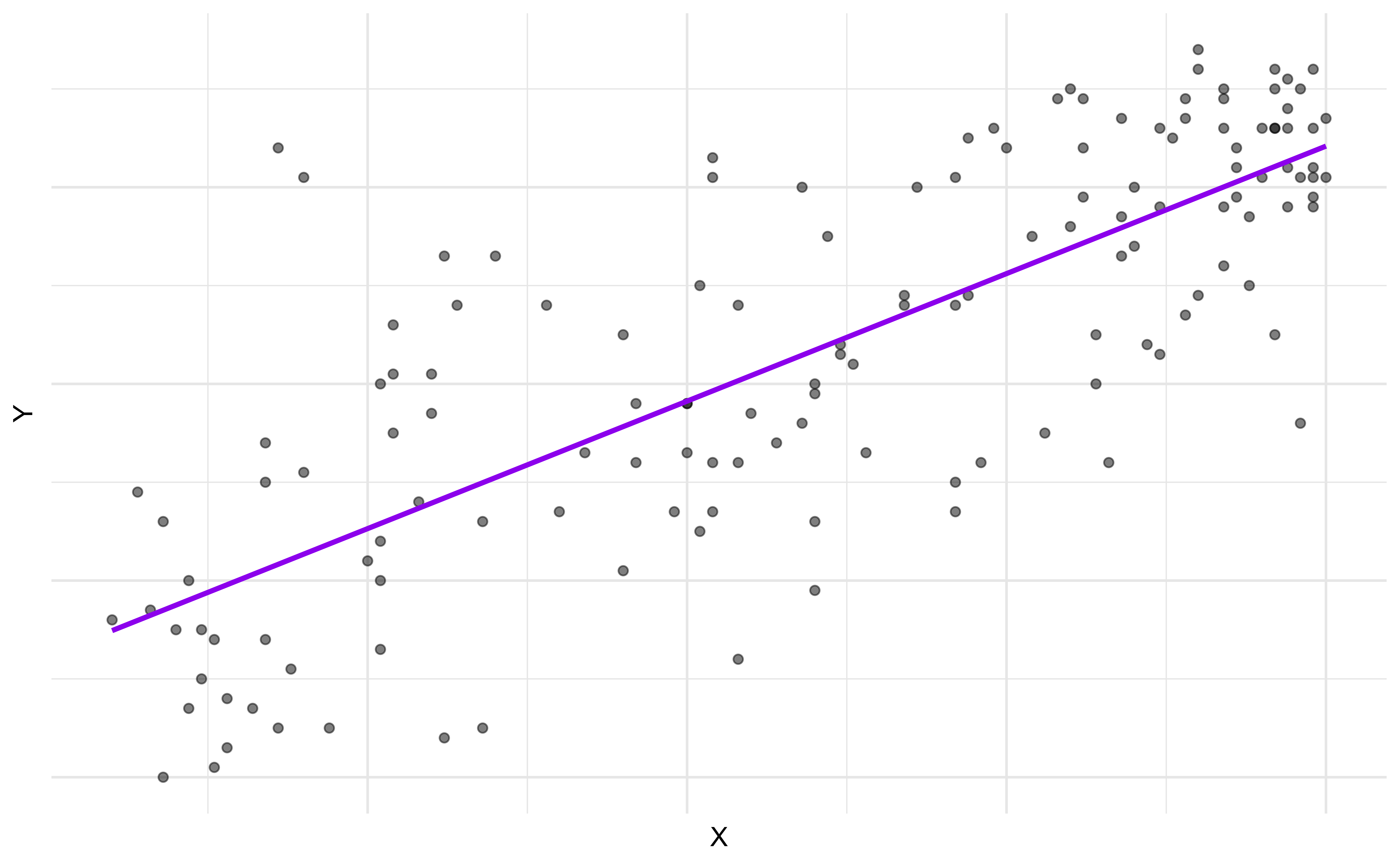
Regression model

$$ \[\begin{aligned} Y &= \color{purple}{\textbf{Model}} + \text{Error} \\[8pt] &= \color{purple}{\mathbf{f(X)}} + \epsilon \\[8pt] &= \color{purple}{\boldsymbol{\mu_{Y|X}}} + \epsilon \end{aligned}\]

$$

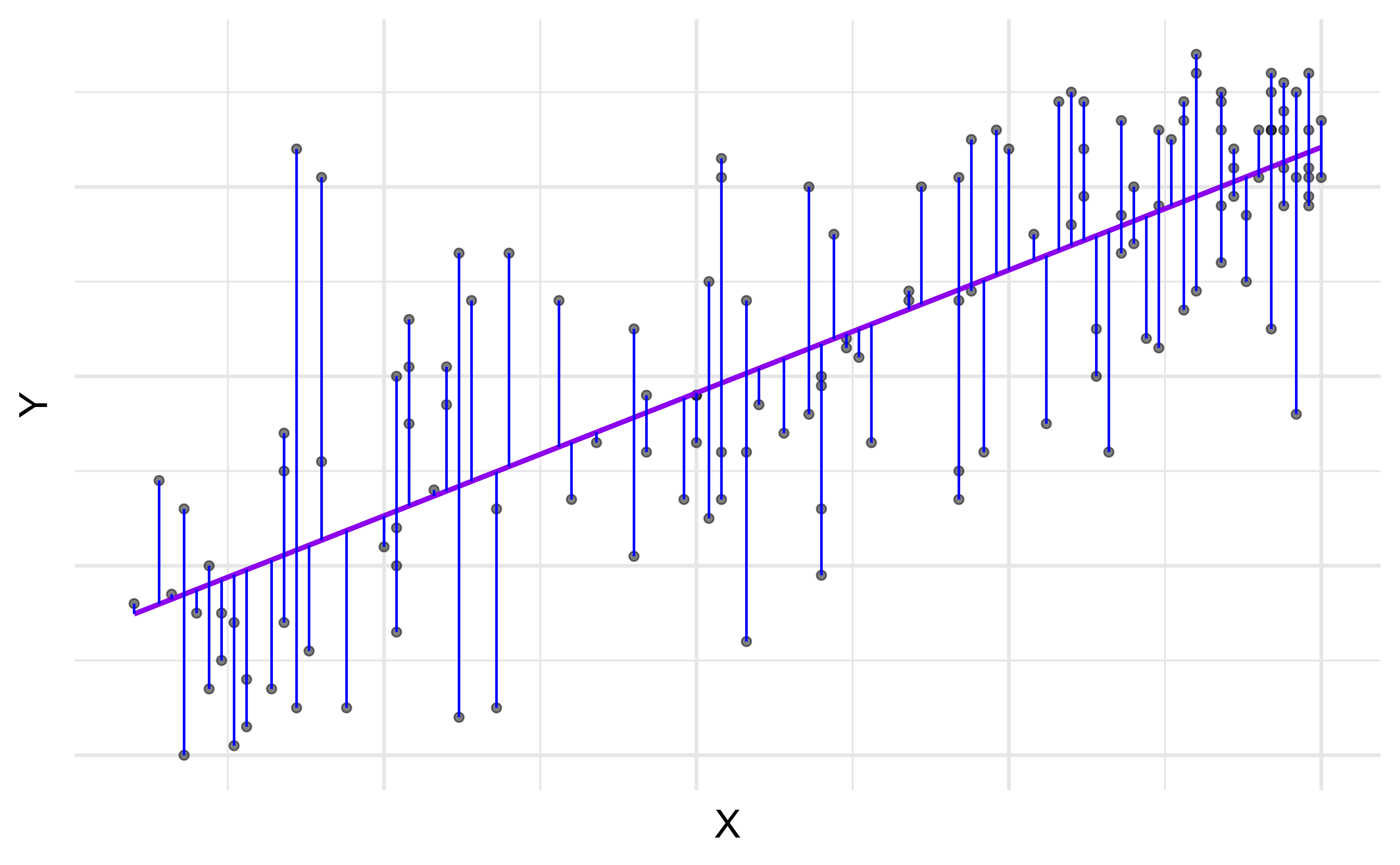
Regression model + residuals

\[\begin{aligned} Y &= \color{purple}{\textbf{Model}} + \color{blue}{\textbf{Error}} \\[8pt] &= \color{purple}{\mathbf{f(X)}} + \color{blue}{\boldsymbol{\epsilon}} \\[8pt] &= \color{purple}{\boldsymbol{\mu_{Y|X}}} + \color{blue}{\boldsymbol{\epsilon}} \\[8pt] \end{aligned}\]

Simple linear regression

Simple linear regression

Use simple linear regression to model the relationthip between a quantitative outcome (\(Y\)) and a single quantitative predictor (\(X\)): \[\Large{Y = \beta_0 + \beta_1 X + \epsilon}\]

• \(\beta_1\): True slope of the relationship between \(X\) and \(Y\)
• \(\beta_0\): True intercept of the relationship between \(X\) and \(Y\)
• \(\epsilon\): Error (residual)

Simple linear regression

\[\Large{\hat{Y} = \hat{\beta}_0 + \hat{\beta}_1 X}\]

• \(\hat{\beta}_1\): Estimated slope of the relationship between \(X\) and \(Y\)
• \(\hat{\beta}_0\): Estimated intercept of the relationship between \(X\) and \(Y\)
• No error term!

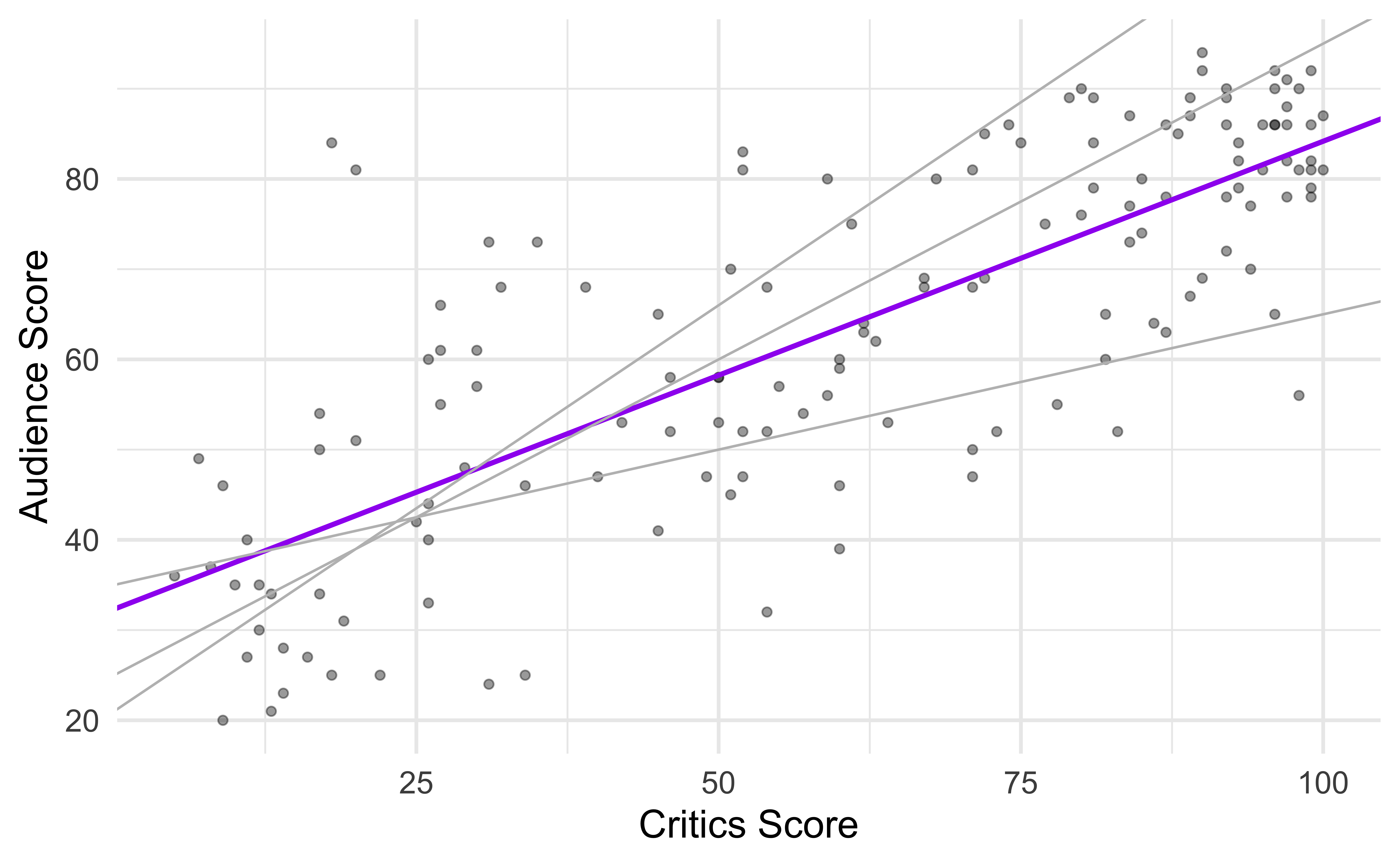
Choosing values for \(\hat{\beta}_1\) and \(\hat{\beta}_0\)

Residuals

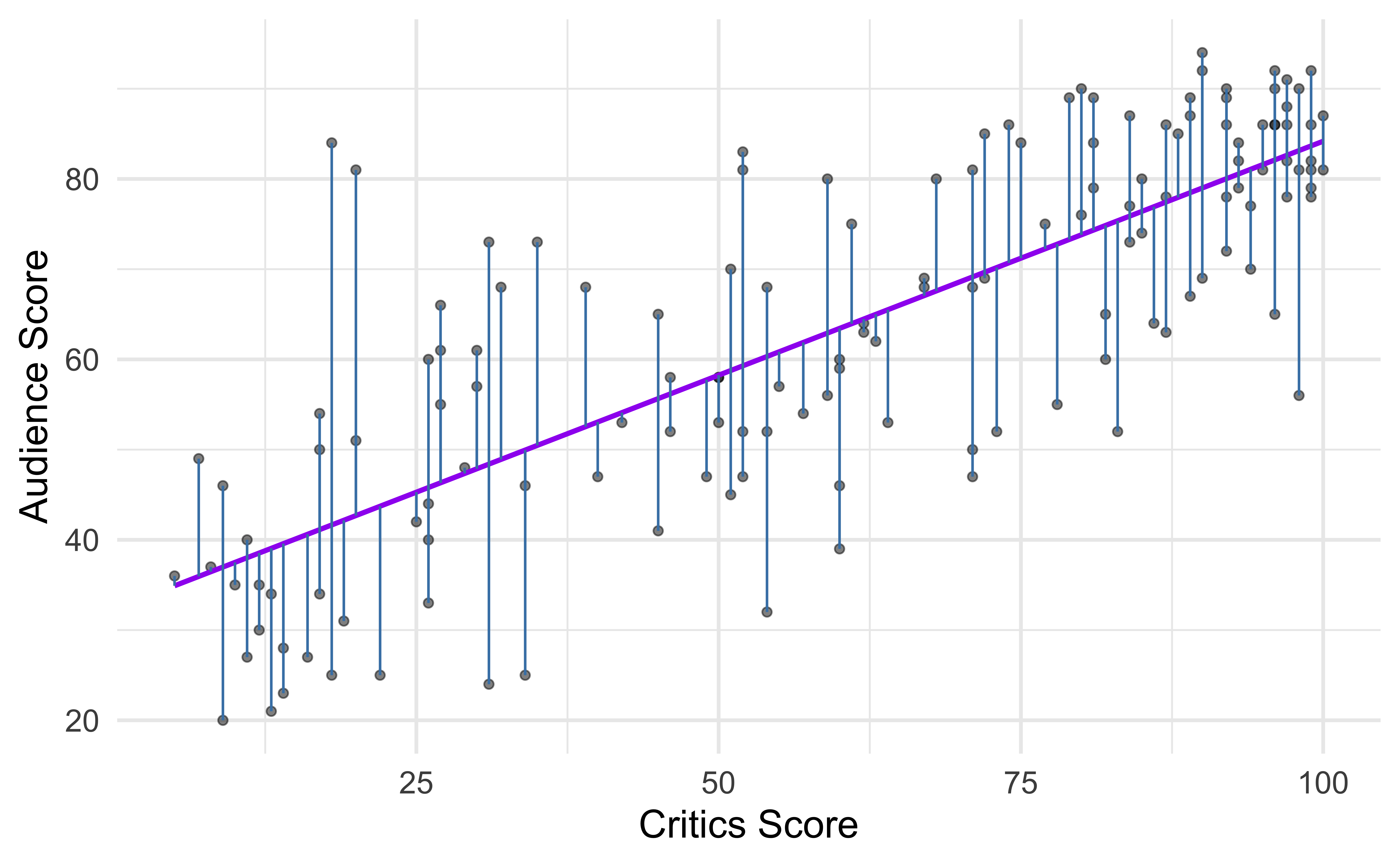
\[\text{residual} = \text{observed} - \text{predicted} = y - \hat{y}\]

Least squares line

• The residual for the \(i^{th}\) observation is

\[e_i = \text{observed} - \text{predicted} = y_i - \hat{y}_i\]

• The sum of squared residuals is

\[e^2_1 + e^2_2 + \dots + e^2_n\]

• The least squares line is the one that minimizes the sum of squared residuals

Slope and intercept

Properties of least squares regression

• The regression line goes through the center of mass point, the coordinates corresponding to average \(X\) and average \(Y\): \(\hat{\beta}_0 = \bar{Y} - \hat{\beta}_1\bar{X}\)

• The slope has the same sign as the correlation coefficient: \(\hat{\beta}_1 = r \frac{s_Y}{s_X}\)

• The sum of the residuals is zero: \(\sum_{i = 1}^n \epsilon_i = 0\)

• The residuals and \(X\) values are uncorrelated

Estimating the slope

\[\large{\hat{\beta}_1 = r \frac{s_Y}{s_X}}\]

\[\begin{aligned} s_X &= 30.1688 \\ s_Y &= 20.0244 \\ r &= 0.7814 \end{aligned}\]

$$ \[\begin{aligned} \hat{\beta}_1 &= 0.7814 \times \frac{20.0244}{30.1688} \\ &= 0.5187\end{aligned}\]

$$

Estimating the intercept

\[\large{\hat{\beta}_0 = \bar{Y} - \hat{\beta}_1\bar{X}}\]

$$ \[\begin{aligned} &\bar{x} = 60.8493 \\ &\bar{y} = 63.8767 \\ &\hat{\beta}_1 = 0.5187 \end{aligned}\]

$$

\[\begin{aligned}\hat{\beta}_0 &= 63.8767 - 0.5187 \times 60.8493 \\ &= 32.3142 \end{aligned}\]

Interpreting the slope

Poll: The slope of the model for predicting audience score from critics score is 32.3142. Which of the following is the best interpretation of this value?

• For every one point increase in the critics score, the audience score goes up by 0.5187 points, on average.
• For every one point increase in the critics score, we expect the audience score to be higher by 0.5187 points, on average.
• For every one point increase in the critics score, the audience score goes up by 0.5187 points.
• For every one point increase in the audience score, the critics score goes up by 0.5187 points, on average.

Interpreting slope & intercept

\[\widehat{\text{audience}} = 32.3142 + 0.5187 \times \text{critics}\]

• Slope: For every one point increase in the critics score, we expect the audience score to be higher by 0.5187 points, on average.
• Intercept: If the critics score is 0 points, we expect the audience score to be 32.3142 points, on average.

Is the intercept meaningful?

✅ The intercept is meaningful in context of the data if

• the predictor can feasibly take values equal to or near zero or
• the predictor has values near zero in the observed data

🛑 Otherwise, it might not be meaningful!

Prediction

Making a prediction

Suppose that a movie has a critics score of 50. According to this model, what is the movie’s predicted audience score?

\[ \begin{aligned} \widehat{\text{audience}} &= 32.3142 + 0.5187 \times \text{critics} \\ &= 32.3142 + 0.5187 \times 50 \\ &= 58.2492 \end{aligned} \]

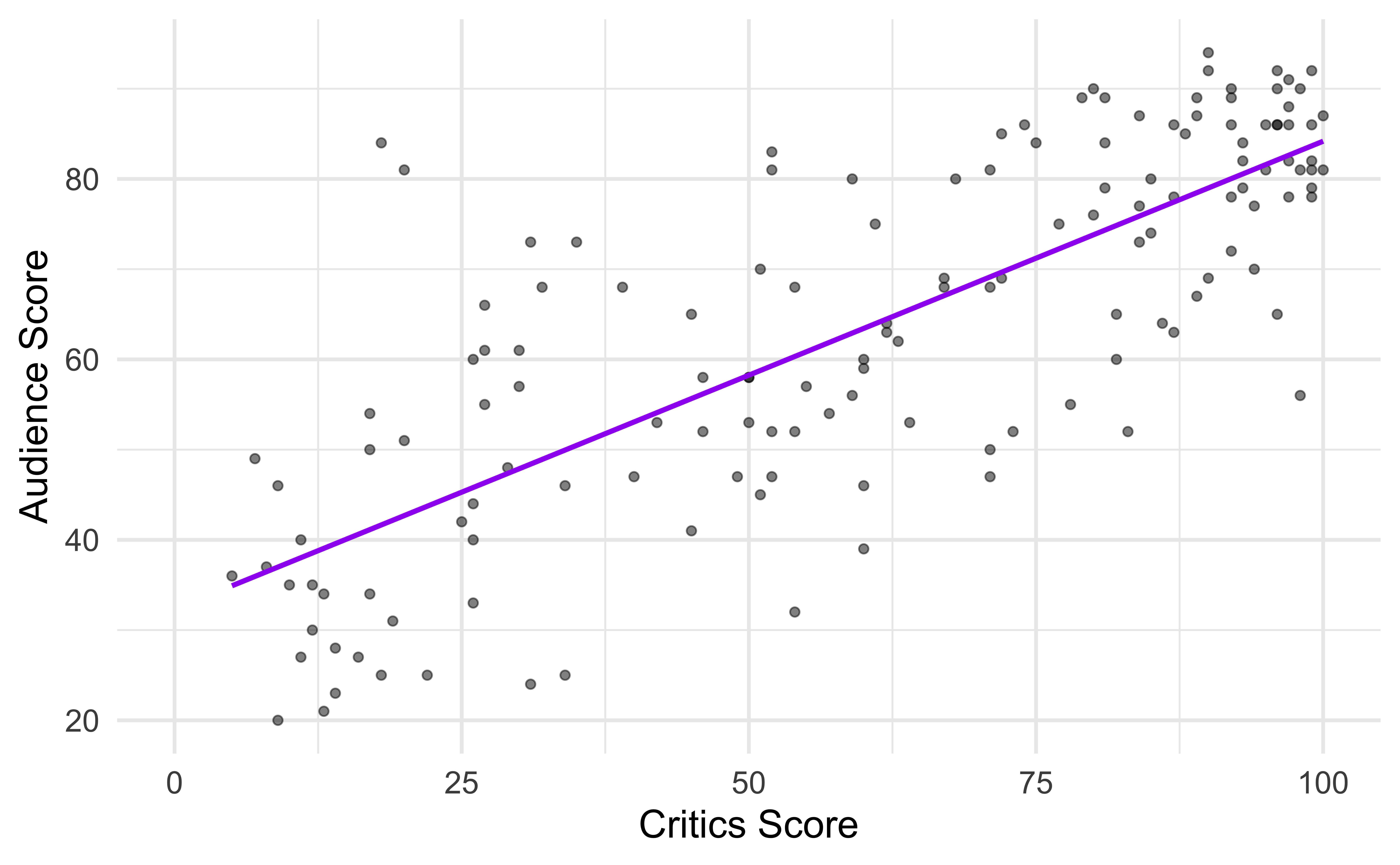
Extrapolation

Extrapolation is prediction outside of the ranged covered by data.

Suppose that a movie has a critics score of 0. According to this model, what is the movie’s predicted audience score?

Recap

Recap

• Used simple linear regression to describe the relationship between a quantitative predictor and quantitative outcome variable.

• Used the least squares method to estimate the slope and intercept.

• We interpreted the slope and intercept.

  • Slope: For every one unit increase in \(x\), we expect y to be higher/lower by \(\hat{\beta}_1\) units, on average.
  • Intercept: If \(x\) is 0, then we expect \(y\) to be \(\hat{\beta}_0\) units.

• Predicted the response given a value of the predictor variable.

• Defined extrapolation and why we should avoid it.