Feature engineering
STA 210 - Summer 2022
Welcome
Announcements
- Check your grades for exam-1
- Go through conceptual questions in homework 2
HW 2 Part 1
Categorical predictors
- Set it to be factor
as.factor - For variable only contains two levels, taking values 0 or 1. No actions needed. Can treat as continuous variable in R, since 1 unit increase equals to difference brought by level 1 compared to baseline level
- Okay to take correlation to depict association
High correlation
- High correlation between predictors: bad
- multicollinearity: large variance -> unreasonable estimator
set.seed(1)
x=rnorm(100,1,1)
epsilon=rnorm(100,0,0.01)
y=2*x+epsilon
dat=tibble(x=x,y=y)
x1=0.8*x+rnorm(100,0.1,0.01)
dat=dat%>%mutate(x1=x1)
lm1=lm(y~x,data = dat)
lm2=lm(y~x+x1,data=dat)
lm3=lm(y~x1+x,data=dat)
Multicollinearity
- No change on point estimator. (rotation)
- Increase se
summary(lm1)
Call:
lm(formula = y ~ x, data = dat)

Residuals:
      Min        1Q    Median        3Q       Max
-0.018768 -0.006138 -0.001395  0.005394  0.023462

Coefficients:
              Estimate Std. Error  t value Pr(>|t|)
(Intercept) -0.0003663  0.0015342   -0.239    0.812
x            1.9999894  0.0010773 1856.534   <2e-16 ***
---
Signif. codes:  0 '***' 0.001 '**' 0.01 '*' 0.05 '.' 0.1 ' ' 1

Residual standard error: 0.009628 on 98 degrees of freedom
Multiple R-squared:      1, Adjusted R-squared:      1
F-statistic: 3.447e+06 on 1 and 98 DF, p-value: < 2.2e-16summary(lm2)
Call:
lm(formula = y ~ x + x1, data = dat)

Residuals:
      Min        1Q    Median        3Q       Max
-0.018455 -0.006465 -0.001507  0.005328  0.023326

Coefficients:
             Estimate Std. Error t value Pr(>|t|)
(Intercept)  0.004224   0.009525   0.443    0.658
x            2.036700   0.075177  27.092   <2e-16 ***
x1          -0.045876   0.093936  -0.488    0.626
---
Signif. codes:  0 '***' 0.001 '**' 0.01 '*' 0.05 '.' 0.1 ' ' 1

Residual standard error: 0.009665 on 97 degrees of freedom
Multiple R-squared:      1, Adjusted R-squared:      1
F-statistic: 1.71e+06 on 2 and 97 DF, p-value: < 2.2e-16summary(lm3)
Call:
lm(formula = y ~ x1 + x, data = dat)

Residuals:
      Min        1Q    Median        3Q       Max
-0.018455 -0.006465 -0.001507  0.005328  0.023326

Coefficients:
             Estimate Std. Error t value Pr(>|t|)
(Intercept)  0.004224   0.009525   0.443    0.658
x1          -0.045876   0.093936  -0.488    0.626
x            2.036700   0.075177  27.092   <2e-16 ***
---
Signif. codes:  0 '***' 0.001 '**' 0.01 '*' 0.05 '.' 0.1 ' ' 1

Residual standard error: 0.009665 on 97 degrees of freedom
Multiple R-squared:      1, Adjusted R-squared:      1
F-statistic: 1.71e+06 on 2 and 97 DF,  p-value: < 2.2e-16
Interpretation on coefficient
- we expect = model predicts = \(\hat{y}\)
- on average = expectation of y
- hold other constant
Cold call since today ! Be prepared !
Topics
- Splitting training set and testing set
- Specify the
recipes(predictors, outcome) stepswithinrecipes(feature engineering)Workflowsto bring together models and recipes- Cook: Fit model and prediction
- Taste it : RMSE and \(R^2\) for model evaluation
- Improve it: Cross validation
Introduction
The Office

Data
The data come from data.world, by way of TidyTuesday
office_ratings <- read_csv(here::here("slides", "data/office_ratings.csv"))
office_ratings
# A tibble: 188 × 6
season episode title imdb_rating total_votes air_date
<dbl> <dbl> <chr> <dbl> <dbl> <date>
1 1 1 Pilot 7.6 3706 2005-03-24
2 1 2 Diversity Day 8.3 3566 2005-03-29
3 1 3 Health Care 7.9 2983 2005-04-05
4 1 4 The Alliance 8.1 2886 2005-04-12
5 1 5 Basketball 8.4 3179 2005-04-19
6 1 6 Hot Girl 7.8 2852 2005-04-26
7 2 1 The Dundies 8.7 3213 2005-09-20
8 2 2 Sexual Harassment 8.2 2736 2005-09-27
9 2 3 Office Olympics 8.4 2742 2005-10-04
10 2 4 The Fire 8.4 2713 2005-10-11
# … with 178 more rowsIMDB ratings
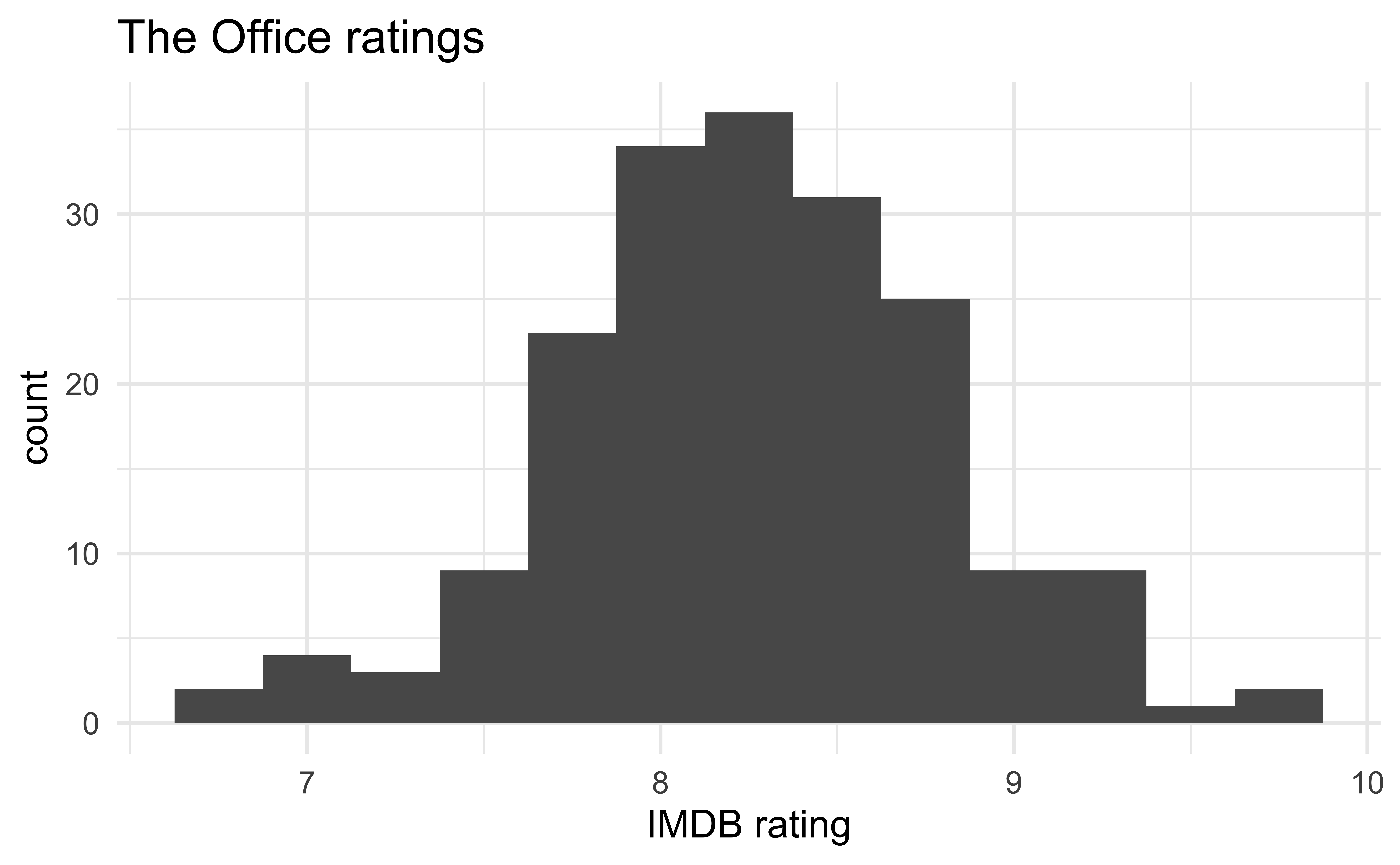
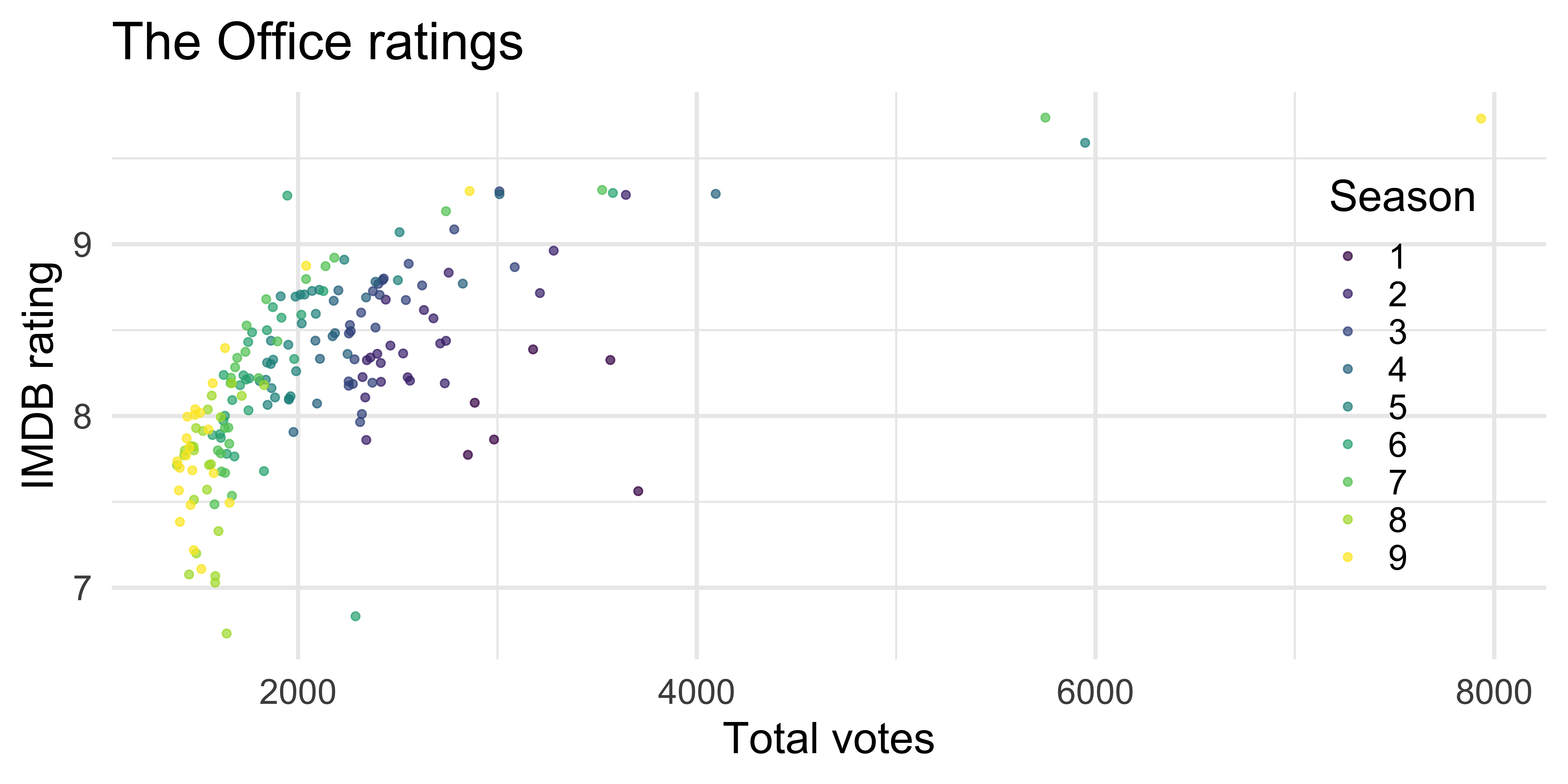
IMDB ratings vs. number of votes
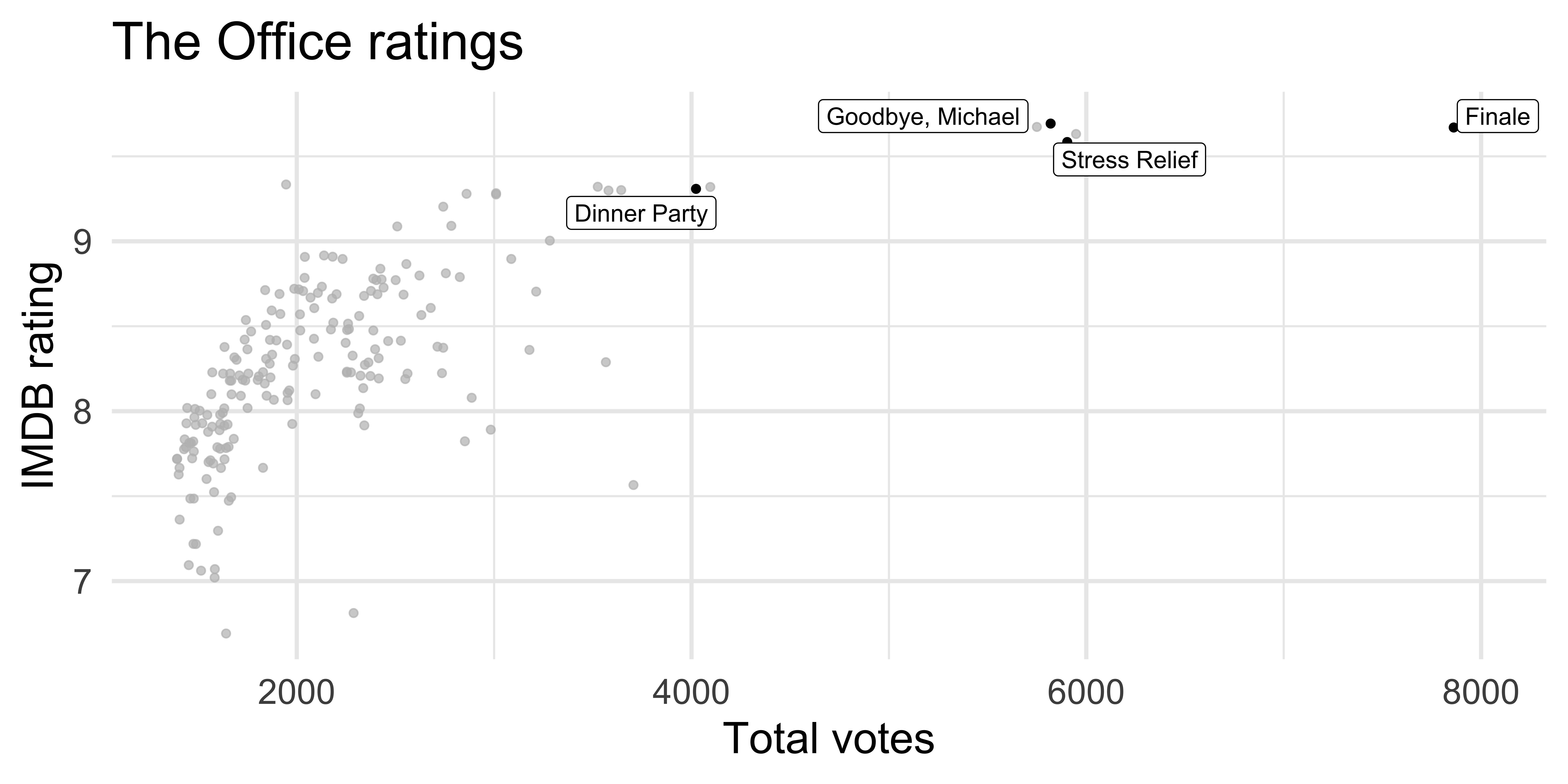
Outliers
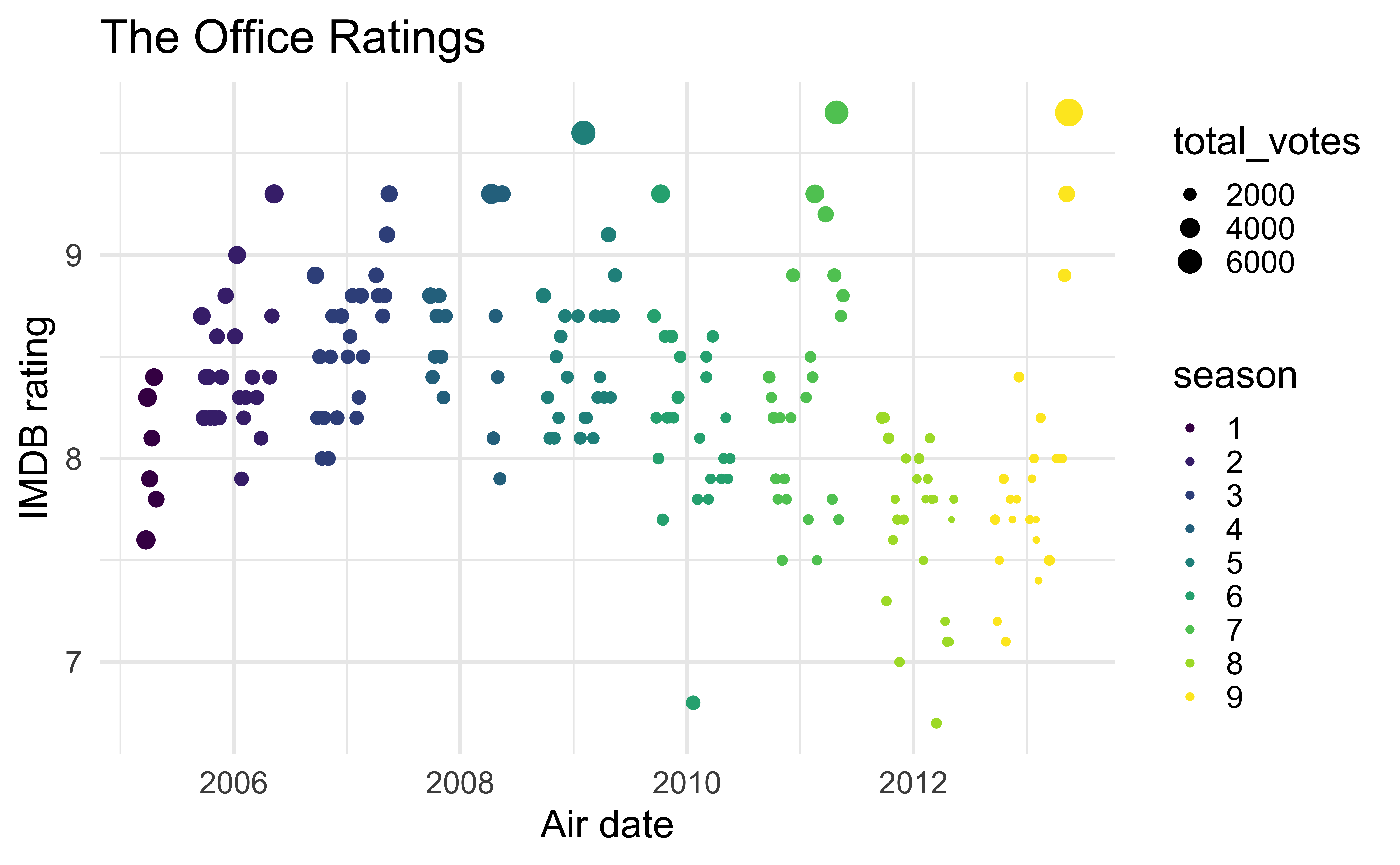
Rating vs. air date

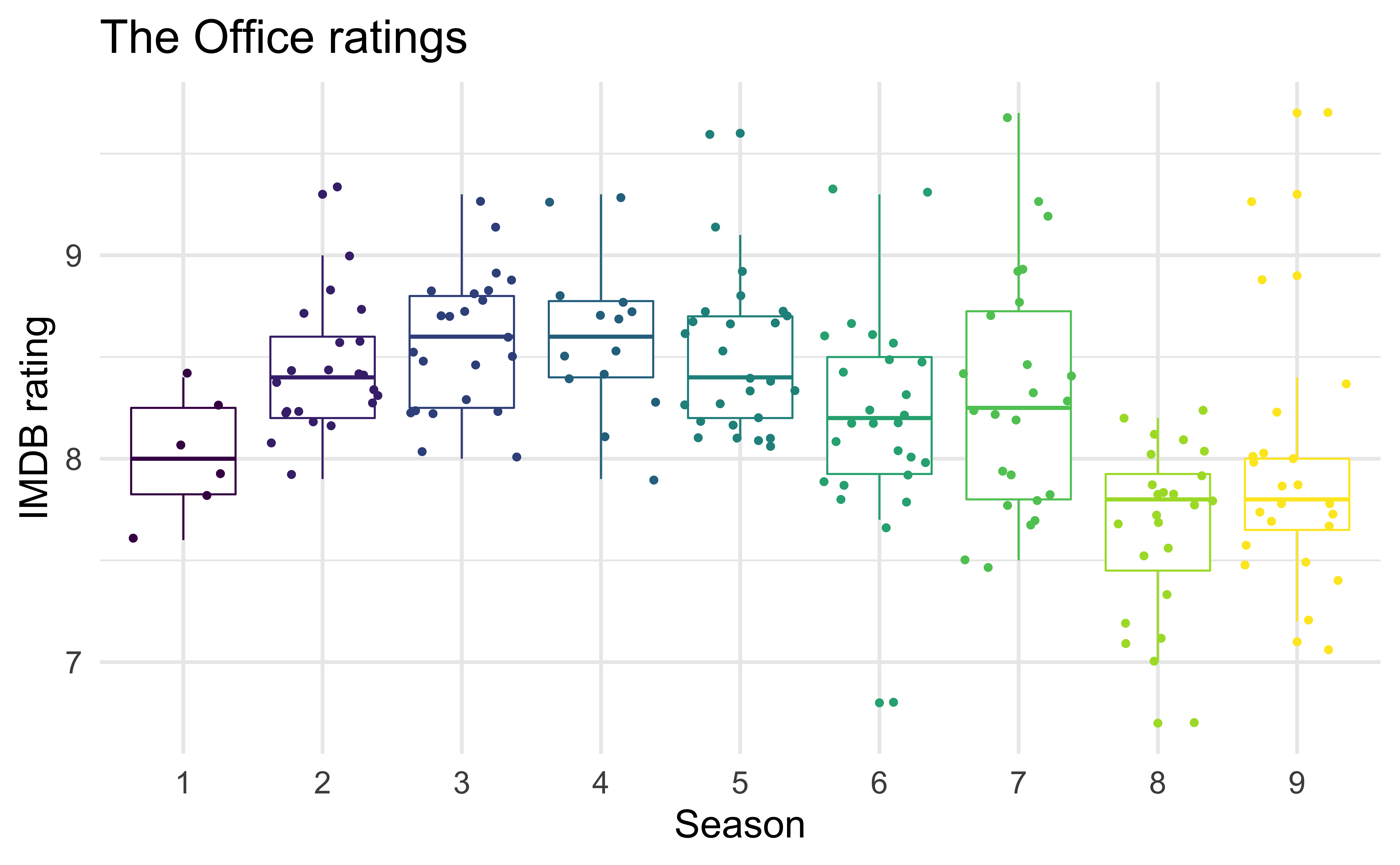
IMDB ratings vs. seasons
Modeling
Train / test
Step 1: Create an initial split:
set.seed(123)
office_split <- initial_split(office_ratings) # prop = 3/4 by default
Step 2: Save training data
office_train <- training(office_split)
dim(office_train)
[1] 141 6Step 3: Save testing data
office_test  <- testing(office_split)
dim(office_test)
[1] 47 6Training data
office_train# A tibble: 141 × 6
season episode title imdb_rating total_votes air_date
<dbl> <dbl> <chr> <dbl> <dbl> <date>
1 8 18 Last Day in Florida 7.8 1429 2012-03-08
2 9 14 Vandalism 7.6 1402 2013-01-31
3 2 8 Performance Review 8.2 2416 2005-11-15
4 9 5 Here Comes Treble 7.1 1515 2012-10-25
5 3 22 Beach Games 9.1 2783 2007-05-10
6 7 1 Nepotism 8.4 1897 2010-09-23
7 3 15 Phyllis' Wedding 8.3 2283 2007-02-08
8 9 21 Livin' the Dream 8.9 2041 2013-05-02
9 9 18 Promos 8 1445 2013-04-04
10 8 12 Pool Party 8 1612 2012-01-19
# … with 131 more rowsFeature engineering
We prefer simple models when possible, but parsimony does not mean sacrificing accuracy (or predictive performance) in the interest of simplicity
Variables that go into the model and how they are represented are just as critical to success of the model
Feature engineering allows us to get creative with our predictors in an effort to make them more useful for our model (to increase its predictive performance)
Variable selection (parsimony) + Variable representation (feature engineering)
Feature engineering : date
Periodic: month or weekday
Feature engineering with dplyr
office_train %>%
  mutate(
    season = as_factor(season),
    month = lubridate::month(air_date),
    wday = lubridate::wday(air_date)
  )
# A tibble: 141 × 8
season episode title imdb_rating total_votes air_date month wday
<fct> <dbl> <chr> <dbl> <dbl> <date> <dbl> <dbl>
1 8 18 Last Day in Flo… 7.8 1429 2012-03-08 3 5
2 9 14 Vandalism 7.6 1402 2013-01-31 1 5
3 2 8 Performance Rev… 8.2 2416 2005-11-15 11 3
4 9 5 Here Comes Treb… 7.1 1515 2012-10-25 10 5
5 3 22 Beach Games 9.1 2783 2007-05-10 5 5
6 7 1 Nepotism 8.4 1897 2010-09-23 9 5
# … with 135 more rowsCan you identify any potential problems with this approach?
Holidays
Modeling workflow
Create a recipe for feature engineering steps to be applied to the training data
Fit the model to the training data after these steps have been applied
Using the model estimates from the training data, predict outcomes for the test data
Evaluate the performance of the model on the test data
Building recipes
Initiate a recipe
Step 1: Alter roles
title isn’t a predictor, but we might want to keep it around as an ID
Step 2: Add features
New features for day of week and month. step_date creates a specification of a recipe step that will convert date data into one or more factor or numeric variables.
Step 3: Add more features
Identify holidays in air_date, then remove air_date
office_rec <- office_rec %>%
step_holiday(
air_date,
holidays = c("USThanksgivingDay", "USChristmasDay", "USNewYearsDay", "USIndependenceDay"),
keep_original_cols = FALSE
)
office_recRecipe
Inputs:
role #variables
ID 1
outcome 1
predictor 4
Operations:
Date features from air_date
Holiday features from air_dateStep 4: Convert numbers to factors
Convert season to factor
Step 5: Make dummy variables
Convert all nominal (categorical) predictors to factors
Step 6: Remove zero variance pred.s
Remove all predictors that contain only a single value
Recipe

Inputs:

      role #variables
        ID          1
   outcome          1
 predictor          4
Operations:
Date features from air_date
Holiday features from air_date
Factor variables from season
Dummy variables from all_nominal_predictors()
Zero variance filter on all_predictors()Steps that may be useful
- Impute data if there is missing data in predictors:
step_impute_knn(all_predictors())
- If intercept is not meaningful and want to center predictors:
step_center(all_numeric_predictors())
- Check other possible steps: recipes
Putting it altogether
office_rec <- recipe(imdb_rating ~ ., data = office_train) %>%
  # make title's role ID
  update_role(title, new_role = "ID") %>%
  # extract day of week and month of air_date
  step_date(air_date, features = c("dow", "month")) %>%
  # identify holidays and add indicators
  step_holiday(
    air_date,
    holidays = c("USThanksgivingDay", "USChristmasDay", "USNewYearsDay", "USIndependenceDay"),
    keep_original_cols = FALSE
  ) %>%
  # turn season into factor
  step_num2factor(season, levels = as.character(1:9)) %>%
  # make dummy variables
  step_dummy(all_nominal_predictors()) %>%
  # remove zero variance predictors
  step_zv(all_predictors())
Putting it altogether
office_recRecipe
Inputs:
role #variables
ID 1
outcome 1
predictor 4
Operations:
Date features from air_date
Holiday features from air_date
Factor variables from season
Dummy variables from all_nominal_predictors()
Zero variance filter on all_predictors()Building workflows
Specify model
office_spec <- linear_reg() %>%
  set_engine("lm")

office_spec
Linear Regression Model Specification (regression)
Computational engine: lm Build workflow
Workflows bring together models and recipes so that they can be easily applied to both the training and test data.
office_wflow <- workflow() %>%
add_model(office_spec) %>%
add_recipe(office_rec)View workflow
office_wflow══ Workflow ════════════════════════════════════════════════════════════════════
Preprocessor: Recipe
Model: linear_reg()
── Preprocessor ────────────────────────────────────────────────────────────────
5 Recipe Steps
• step_date()
• step_holiday()
• step_num2factor()
• step_dummy()
• step_zv()
── Model ───────────────────────────────────────────────────────────────────────
Linear Regression Model Specification (regression)

Computational engine: lm Fit model
Fit model to training data
Cold Call !
office_fit <- office_wflow %>%
  fit(data = office_train)

tidy(office_fit)
# A tibble: 21 × 5
term estimate std.error statistic p.value
<chr> <dbl> <dbl> <dbl> <dbl>
1 (Intercept) 6.40 0.510 12.5 1.51e-23
2 episode -0.00393 0.0171 -0.230 8.18e- 1
3 total_votes 0.000375 0.0000414 9.07 2.75e-15
4 season_X2 0.811 0.327 2.48 1.44e- 2
5 season_X3 1.04 0.343 3.04 2.91e- 3
6 season_X4 1.09 0.295 3.70 3.32e- 4
7 season_X5 1.08 0.348 3.11 2.34e- 3
8 season_X6 1.00 0.367 2.74 7.18e- 3
9 season_X7 1.02 0.352 2.89 4.52e- 3
10 season_X8 0.497 0.348 1.43 1.55e- 1
# … with 11 more rowsSo many predictors!
Model fit summary
Print all the predictors w/o folding any
tidy(office_fit) %>% print(n = 21)# A tibble: 21 × 5
term estimate std.error statistic p.value
<chr> <dbl> <dbl> <dbl> <dbl>
1 (Intercept) 6.40 0.510 12.5 1.51e-23
2 episode -0.00393 0.0171 -0.230 8.18e- 1
3 total_votes 0.000375 0.0000414 9.07 2.75e-15
4 season_X2 0.811 0.327 2.48 1.44e- 2
5 season_X3 1.04 0.343 3.04 2.91e- 3
6 season_X4 1.09 0.295 3.70 3.32e- 4
7 season_X5 1.08 0.348 3.11 2.34e- 3
8 season_X6 1.00 0.367 2.74 7.18e- 3
9 season_X7 1.02 0.352 2.89 4.52e- 3
10 season_X8 0.497 0.348 1.43 1.55e- 1
11 season_X9 0.621 0.345 1.80 7.41e- 2
12 air_date_dow_Tue 0.382 0.422 0.904 3.68e- 1
13 air_date_dow_Thu 0.284 0.389 0.731 4.66e- 1
14 air_date_month_Feb -0.0597 0.132 -0.452 6.52e- 1
15 air_date_month_Mar -0.0752 0.156 -0.481 6.31e- 1
16 air_date_month_Apr 0.0954 0.177 0.539 5.91e- 1
17 air_date_month_May 0.156 0.213 0.734 4.64e- 1
18 air_date_month_Sep -0.0776 0.223 -0.348 7.28e- 1
19 air_date_month_Oct -0.176 0.174 -1.01 3.13e- 1
20 air_date_month_Nov -0.156 0.149 -1.05 2.98e- 1
21 air_date_month_Dec 0.170 0.149 1.14 2.55e- 1Evaluate model
Make predictions for training data
office_train_pred <- predict(office_fit, office_train) %>%
  bind_cols(office_train %>% select(imdb_rating, title))

office_train_pred
# A tibble: 141 × 3
.pred imdb_rating title
<dbl> <dbl> <chr>
1 7.57 7.8 Last Day in Florida
2 7.77 7.6 Vandalism
3 8.31 8.2 Performance Review
4 7.67 7.1 Here Comes Treble
5 8.84 9.1 Beach Games
6 8.33 8.4 Nepotism
7 8.46 8.3 Phyllis' Wedding
8 8.14 8.9 Livin' the Dream
9 7.87 8 Promos
10 7.74 8 Pool Party
# … with 131 more rowsR-squared
Percentage of variability in the IMDB ratings explained by the model.
rsq(office_train_pred, truth = imdb_rating, estimate = .pred)# A tibble: 1 × 3
.metric .estimator .estimate
<chr> <chr> <dbl>
1 rsq standard 0.670Are models with high or low \(R^2\) more preferable?
RMSE
An alternative model performance statistic: root mean square error.
\[ RMSE = \sqrt{\frac{\sum_{i = 1}^n (y_i - \hat{y}_i)^2}{n}} \]
rmse(office_train_pred, truth = imdb_rating, estimate = .pred)# A tibble: 1 × 3
.metric .estimator .estimate
<chr> <chr> <dbl>
1 rmse standard 0.302Are models with high or low RMSE are more preferable?
Interpreting RMSE
Is this RMSE considered low or high?
rmse(office_train_pred, truth = imdb_rating, estimate = .pred)# A tibble: 1 × 3
.metric .estimator .estimate
<chr> <chr> <dbl>
1 rmse standard 0.302Depends…
office_train %>%
  summarise(min = min(imdb_rating), max = max(imdb_rating))
# A tibble: 1 × 2
min max
<dbl> <dbl>
1 6.7 9.7But, really…
who cares about predictions on training data?
Make predictions for testing data
office_test_pred <- predict(office_fit, office_test) %>%
  bind_cols(office_test %>% select(imdb_rating, title))

office_test_pred
# A tibble: 47 × 3
.pred imdb_rating title
<dbl> <dbl> <chr>
1 8.03 8.3 Diversity Day
2 7.98 7.9 Health Care
3 8.41 8.4 The Fire
4 8.35 8.2 Halloween
5 8.35 8.4 E-Mail Surveillance
6 8.68 9 The Injury
7 8.32 7.9 The Carpet
8 8.93 9.3 Casino Night
9 8.80 8.9 Gay Witch Hunt
10 8.37 8.2 Initiation
# … with 37 more rowsEvaluate performance for testing data
RMSE of model fit to testing data
rmse(office_test_pred, truth = imdb_rating, estimate = .pred)# A tibble: 1 × 3
.metric .estimator .estimate
<chr> <chr> <dbl>
1 rmse standard 0.411R-sq of model fit to testing data
rsq(office_test_pred, truth = imdb_rating, estimate = .pred)# A tibble: 1 × 3
.metric .estimator .estimate
<chr> <chr> <dbl>
1 rsq standard 0.468Training vs. testing
| metric | train | test | comparison |
|---|---|---|---|
| RMSE | 0.302 | 0.411 | RMSE lower for training |
| R-squared | 0.67 | 0.468 | R-squared higher for training |
Evaluating performance on training data
The training set does not have the capacity to be a good arbiter of performance.
It is not an independent piece of information; predicting the training set can only reflect what the model already knows.
Suppose you give a class a test, then give them the answers, then provide the same test. The student scores on the second test do not accurately reflect what they know about the subject; these scores would probably be higher than their results on the first test.