library(tidyverse)
library(tidymodels)
library(knitr)
library(palmerpenguins)HW 2 - Multiple linear regression
Due Sunday, May 29, 11:59pm on Gradescope
Introduction
In this assignment, you’ll get to put into practice the multiple linear regression skills you’ve developed.
Learning goals
In this assignment, you will…
- Fit and interpret multiple linear regression models with main and interaction effects.
- Compare multiple linear regression models.
- Reason around multiple linear regression concepts.
- Continue developing a workflow for reproducible data analysis.
Getting started
Your repo for this assignment is at github.com/STA210-Summer22 and starts with the prefix hw-2. For more detailed instructions on getting started, see HW 1.
Packages
The following packages will be used in this assignment. You can add other packages as needed.
Part 1 - Conceptual
Dealing with categorical predictors. Two friends, Elliott and Adrian, want to build a model predicting typing speed (average number of words typed per minute) from whether the person wears glasses or not. Before building the model they want to conduct some exploratory analysis to evaluate the strength of the association between these two variables, but they’re in disagreement about how to evaluate how strongly a categorical predictor is associated with a numerical outcome. Elliott claims that it is not possible to calculate a correlation coefficient to summarize the relationship between a categorical predictor and a numerical outcome, however they’re not sure what a better alternative is. Adrian claims that you can recode a binary predictor as a 0/1 variable (assign one level to be 0 and the other to be 1), thus converting it to a numerical variable. According to Adrian, you can then calculate the correlation coefficient between the predictor and the outcome. Who is right: Elliott or Adrian? If you pick Elliott, can you suggest a better alternative for evaluating the association between the categorical predictor and the numerical outcome?
High correlation, good or bad? Two friends, Frances and Annika, are in disagreement about whether high correlation values are always good in the context of regression. Frances claims that it’s desirable for all variables in the dataset to be highly correlated to each other when building linear models. Annika claims that while it’s desirable for each of the predictors to be highly correlated with the outcome, it is not desirable for the predictors to be highly correlated with each other. Who is right: Frances, Annika, both, or neither? Explain your reasoning using appropriate terminology.
Training for the 5K. Nico signs up for a 5K (a 5,000 metre running race) 30 days prior to the race. They decide to run a 5K every day to train for it, and each day they record the following information:
days_since_start(number of days since starting training),days_till_race(number of days left until the race),mood(poor, good, awesome),tiredness(1-not tired to 10-very tired), andtime(time it takes to run 5K, recorded as mm:ss). Top few rows of the data they collect is shown below.days_since_start days_till_race mood tiredness time 1 29 good 3 25:45 2 28 poor 5 27:13 3 27 awesome 4 24:13 … … … … … Using these data Nico wants to build a model predicting
timefrom the other variables. Should they include all variables shown above in their model? Why or why not?Multiple regression fact checking. Determine which of the following statements are true and false. For each statement that is false, explain why it is false.
If predictors are colinear, then removing one variable will have no influence on the point estimate of another variable’s coefficient.
Suppose a numerical predictor \(x\) has a coefficient of \(\hat{\beta}_1 = 2.5\) in a multiple regression model. Suppose also that the first observation has \(x_{1,1} = 7.2\), the second observation has a value of \(x_{2,1} = 8.2\), and these two observations have the same values for all other predictors. Then the predicted value of the second observation will be 2.5 higher than the prediction of the first observation based on the multiple regression model.
If a regression model’s first predictor has a coefficient of \(\hat{\beta}_1 = 5.7\) and if we are able to influence the data so that an observation will have its \(x_1\) be 1 larger than it would otherwise, the value \(\hat{y}_1\) for this observation would increase by 5.7.
Part 2 - Palmer penguins
Data were collected and made available by Dr. Kristen Gorman and the Palmer Station, Antarctica LTER, a member of the Long Term Ecological Research Network. (Gorman, Williams, and Fraser 2014)

These data can be found in the palmerpenguins package. We’re going to be working with the penguins dataset from this package. The dataset contains data for 344 penguins. There are 3 different species of penguins in this dataset, collected from 3 islands in the Palmer Archipelago, Antarctica.
- Body mass. Our first goal is to fit a model predicting body mass (which is more difficult to measure) from bill length, bill depth, flipper length, species, and sex.
Fit a model predicting body mass (which is more difficult to measure) from the other variables listed above.
Write the equation of the regression model.
Interpret each one of the slopes in this context.
Calculate the residual for a male Adelie penguin that weighs 3750 grams with the following body measurements:
bill_length_mm= 39.1,bill_depth_mm= 18.7,flipper_length_mm= 181. Does the model overpredict or underpredict this penguin’s weight?Find the \(R^2\) of this model and interpret this value in context of the data and the model.
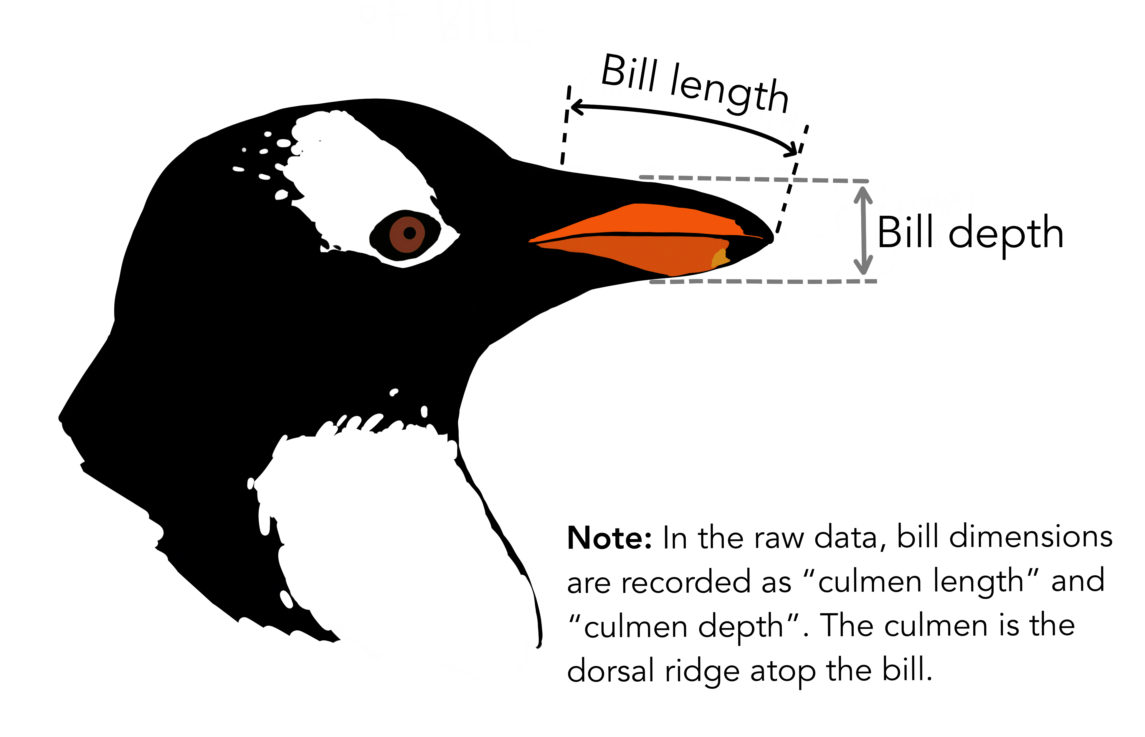
- Bill depth. Next we’ll be focusing on bill depth and bill length and also considering species.
Fit a model predicting bill depth from bill length. Find the adjusted R-squared, AIC, and BIC for this model.
Then, add a new predictor: species. Fit another model predicting bill depth from bill length and species. Find the adjusted R-squared, AIC, and BIC for this model.
Finally, add one more predictor: the interaction between bill length and species. Find the adjusted R-squared, AIC, and BIC for this model.
Using the three criteria you recorded for these three models, and with the goal of parsimony, which model is the “best” for predicting bill depth from bill length and/or species. Explain your reasoning.
Create a visualization representing your model from part a. Hint: Make a scatterplot of bill depth vs. bill length and add the linear model.
Create a visualization representing your model from part b. Hint: Same as part (e), but think about how many lines to plot and whether their slopes should be the same or different.
Create a visualization representing your model from part c. Hint: Same as part (f), but think about how many lines to plot and whether their slopes should be the same or different.
Based on your visualizations from parts e - g, and with the goal of parsimony, is your answer for which model is the “best” for predicting bill depth from bill length and/or species the same as your answer in part d? Explain your reasoning.
Part 3 - Perceived threat of Covid-19
Garbe, Rau, and Toppe (2020), published in June 2020, aims to examine the relationship between personality traits, perceived threat of Covid-19 and stockpiling toilet paper. For this study titled Influence of perceived threat of Covid-19 and HEXACO personality traits on toilet paper stockpiling, researchers conducted an online survey March 23 - 29, 2020 and used the results to fit multiple linear regression models to draw conclusions about their research questions. From their survey, they collected data on adults across 35 countries. Given the small number of responses from people outside of the United States, Canada, and Europe, only responses from people in these three locations were included in the regression analysis.
Let’s consider their results for the model looking at the effect on perceived threat of Covid-19. The model can be found on page 6 of the paper. The perceived threat of Covid was quantified using the responses to the following survey question:
How threatened do you feel by Coronavirus? [Users select on a 10-point visual analogue scale (Not at all threatened to Extremely Threatened)]
Interpret the coefficient of Age (0.072) in the context of the analysis.
Interpret the coefficient of Place of residence in the context of the analysis.
The model includes an interaction between Place of residence and Emotionality (capturing differential tendencies in to worry and be anxious).
What does the coefficient for the interaction (0.101) mean in the context of the data?
Interpret the estimated effect of Emotionality for a person who lives in the US/Canada.
Interpret the estimated effect of Emotionality for a person who lives in Europe.
Submission
Warning
Before you wrap up the assignment, make sure all documents are updated on your GitHub repo. We will be checking these to make sure you have been practicing how to commit and push changes.
Remember – you must turn in a PDF file to the Gradescope page before the submission deadline for full credit.
To submit your assignment:
- Go to http://www.gradescope.com and click Log in in the top right corner.
- Click School Credentials ➡️ Duke NetID and log in using your NetID credentials.
- Click on your STA 210 course.
- Click on the assignment, and you’ll be prompted to submit it.
- Mark the pages associated with each exercise. All of the pages of your lab should be associated with at least one question (i.e., should be “checked”).
- Select the first page of your PDF submission to be associated with the “Workflow & formatting” section.
Grading
Total points available: 50 points.
| Component | Points |
|---|---|
| Ex 1 - 9 | 45 |
| Workflow & formatting | 51 |
References
Garbe, Lisa, Richard Rau, and Theo Toppe. 2020. “Influence of Perceived Threat of Covid-19 and HEXACO Personality Traits on Toilet Paper Stockpiling.” Edited by Valerio Capraro. PLOS ONE 15 (6): e0234232. https://doi.org/10.1371/journal.pone.0234232.
Gorman, Kristen B., Tony D. Williams, and William R. Fraser. 2014. “Ecological Sexual Dimorphism and Environmental Variability Within a Community of Antarctic Penguins (Genus Pygoscelis).” PLOS ONE 9 (3): e90081. https://doi.org/10.1371/journal.pone.0090081.
Footnotes
The “Workflow & formatting” grade is to assess the reproducible workflow. This includes having at least 3 informative commit messages and updating the name and date in the YAML.↩︎