AE 3: Duke Forest houses

Checking model conditions

Important

Go to the course GitHub organization and locate the repo titled ae-3-YOUR_GITHUB_USERNAME to get started.

Packages

library(tidyverse)
library(tidymodels)
library(openintro)
library(knitr)

Predict sale price from area

df_fit <- linear_reg() %>%
  set_engine("lm") %>%
  fit(price ~ area, data = duke_forest)

tidy(df_fit) %>%
  kable(digits = 2)

term	estimate	std.error	statistic	p.value
(Intercept)	116652.33	53302.46	2.19	0.03
area	159.48	18.17	8.78	0.00

Model conditions

Exercise 1

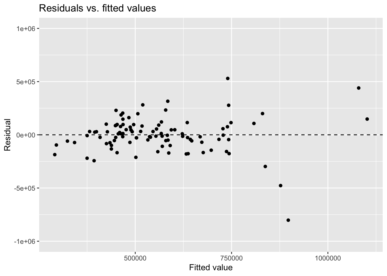
The following code produces the residuals vs. fitted values plot for this model. Comment out the layer that defines the y-axis limits and re-create the plot. How does the plot change? Why might we want to define the limits explicitly?

df_aug <- augment(df_fit$fit)

ggplot(df_aug, aes(x = .fitted, y = .resid)) +
  geom_point() +
  geom_hline(yintercept = 0, linetype = "dashed") +
  ylim(-1000000, 1000000) +
  labs(
    x = "Fitted value", y = "Residual",
    title = "Residuals vs. fitted values"
  )

Exercise 2

Improve how the values on the axes of the plot are displayed by modifying the code below.

Hint: use scale_continuous()

ggplot(df_aug, aes(x = .fitted, y = .resid)) +
  geom_point() +
  geom_hline(yintercept = 0, linetype = "dashed") +
  ylim(-1000000, 1000000) +
  labs(
    x = "Fitted value", y = "Residual",
    title = "Residuals vs. fitted values"
  )